Open Journal of Applied Sciences, 2013, 3, 84-88
doi:10.4236/ojapps.2013.31B1017 Published Online April 2013 (http://www.scirp.org/journal/ojapps)
Reliability of Attenuation Properties Recovery for
Viscoelastic Media
Ekaterina Efimova, Vladimir Cheverda
The laboratory “Numerical methods of inversion of geophysical wavefiel ds”, A.A. Trofimuk Institute of Petroleum
Geology and Geophysics SB RAS. Novosibirsk, Russia
Email: EfimovaES@ipgg.sbras.ru
Received 2013
ABSTRACT
The inverse problem of seismology for media with attenuation is considered in this paper. Generalized Standard Linear
Solid is used to describe viscoelastic media. In the numerical solution certain parameterizations can be coupled, it
means that true heterogeneity of the only one of parameters can be restored only as a perturbation of another. This is
why important to investigate reliability of parameters recovery. By using method based on diffraction patterns it is pos-
sible to see whether the parameters are coupled. Singular value decomposition was used to study the possibility of re-
covering the parameters in practice. It was investigated th e possibility of reconstructing of the d ensity, impedances and
attenuation properties. Coupling appears on the attenuation properties and impedances separately corresponding to the
P-wave and S-wave. It is also should be noted that coupling decreases with increasing frequency range and the condi-
tion num ber.
Keywords: Viscoelasticity; Seismic Attenuation; Inverse Theory; Wave Propagation; Si n gul ar Value Decomposi t i on;
Diffraction Patterns
1. Introduction
The main theme of the work is recovery of characteristics
of viscoelastic media. For this purpose was considered
numerical solution of two-dimensional inverse problem
of seismology using the information recorded in the re-
ceivers located on the surface of the Earth. It is known
that a numerical model of viscoelastic media describes
the geological structures, in particular hydrocarbon res-
ervoirs. And the attenuation properties depend on the
composit i on of the fluid.
But there appears coupling of parameters of the me-
dium in the numerical formulation of the problem that
will be discussed in this article. Coupling of parameters
means that the true heterogeneity of only one parameter
would restore as a perturbation of other in the numerical
solution. So if you use coupled parameters, yo ur solution
will be incorrect. Therefore, we need to find uncoupled
set of parameters before developing and implementation
of the algorithm.
Determination the possibility of uncoupled reconstruc-
tion of the parameters of a viscoelastic medium, such as
density, elastic impedances and attenuation properties is
the subject of this research.
This problem was considered in other papers, in par-
ticular, in [1], the problem was solved for the case of
media with a velocity close to a constant value. There
was also shown the inability simultaneous recovery of
the velocity and attenuation properties in viscoelastic
media without additiona l conditions [2].
2. Numerical Description of Viscoelastic
Media
State equation provides the relationship between stresses
and strains at the same time for ideal elastic media. But
this is not true in viscoelastic media, which possess at-
tenuation that caused by memory of the material. For
such media stress state depends on all past states of
strains and the state equation can be expressed with the
use of the generalized Hooke's law. Media with attenua-
tion mathematically can be described by the system of
equations:
/*
/( )/2
(,)(,)/(,) .
t
kl ijkl
utdiv f
tuu
x
txGxt
ij

d
 

 

 
 (1)
2.1. Generalized Standard Linear Solid
Numerical resolution of such integral-differential system
is very troublesome, so it is proposed to use Standard
Copyright © 2013 SciRes. OJAppS
E. EFIMOVA, V. CHEVERDA 85
Linear Solid (SLS) – superposition of Maxwell medium
and Kelvin-Voigt medium, to represent state equation in
a differential form. The degree of attenuation(see in [3])
of a viscoelastic material is given by a Quality Factor Q
(QF). Quality factor - the number of wavelengths a wave
can propagate through a medium before its amplitude
was decreased in times.
exp( )
It is known that a model that describes real geologic
medium has constant quality factor in dependence of
time frequency over the frequency range [4]. As one can
see SLS does not satisfy this condition, in contrast to the
further considered Generalized Standard Linear Solid
(GSLS) [5] – a combination of several SLSs. Hooke's
law in GSLS rewrites in the form of equations:

,
,
1
//
Lj
j
lllR l
Mtt

 

 
where L – is a number of SLS (further L=2);
,
ll
- constants, that are called relaxation times of
stresses and strains respectively; 2
R
M


- deformation modulus,
where
for
P-wave, , for S-wave,
R
M
- Lame parameters .
Using GSLS model quality factor in the frequency
domain can be rewritten as the equation (see [6]):
,
2
22 2
11
2
1
111
(
QLL
ll
l
l
ll
l
L


)
l
 
 








where the
is a frequency .
To determine the relaxation times in [6] it is proposed
to use
method by introducing the parameters of
attenuation - variables ,
s
p
P, S (corresponding to P-,
S-waves), that describe the level of attenuation in the
medium. It should be noted that if we know the parame-
ters of attenuation we have the only way to determine the
quality factor:
2
22
1
2
12, .
11
ps
ll
LL
ps
ll
l
QQ


  
2
l





So in further considerations we will use the parameters
of attenuation rather than Quality Factor because of sev-
eral advantages of the
method that is listed in [6].
2.2. Linearization
After application of GSLS and the
m
(DB
method system
of equations (1) can be regarded as a nonlinear opera-
tional equation: , where - the parame-
ters of the medium, - observation data, is an
operator from the space of models to the data space. It is
suggested to use Newton's method:
() obs
Bm u
obs
uB
1kk
)k
m mm
 
where ia a - Frechet derivative of
the operator , is model of the medium on the
k-th step.
)(,
obs k
uBm
BDB
k
m
We mean that the parameters of the medium can be
expressed as the sum of the constant components 0
m
and small perturbations m
:0
mm m

 
uu ; then the
total wave field will be presented as 0u

 
, where
0
u
- propagating in a homogeneous medium wave, and
u
- component generated by small perturbations of pa-
rameters. Small quantities of the second order are ig-
nored in the linearization.
3. Coupling Parameters
Coupling between parameters means that in solution of
the problem true heterogeneity of one parameter can be
mistakenly identified as heterogeneity of another pa-
rameter [7]. The presence of coupling indicates wrong
solution. Therefore, we will focus on methods identifying
coupling sets of parameters.
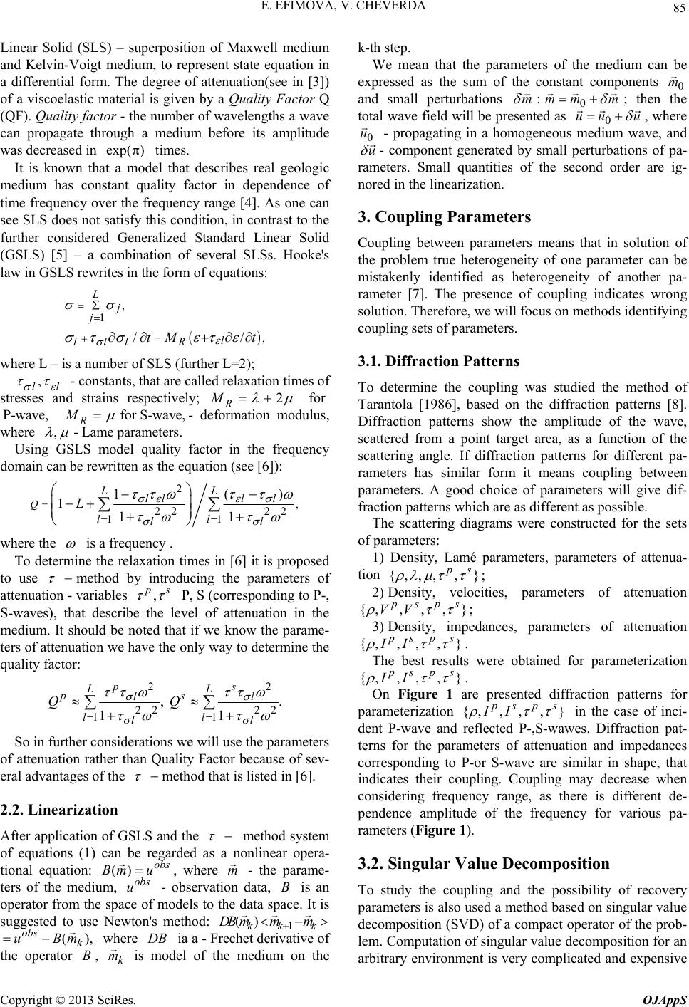
3.1. Diffraction Patterns
To determine the coupling was studied the method of
Tarantola [1986], based on the diffraction patterns [8].
Diffraction patterns show the amplitude of the wave,
scattered from a point target area, as a function of the
scattering angle. If diffraction patterns for different pa-
rameters has similar form it means coupling between
parameters. A good choice of parameters will give dif-
fraction patterns which are as different as possible.
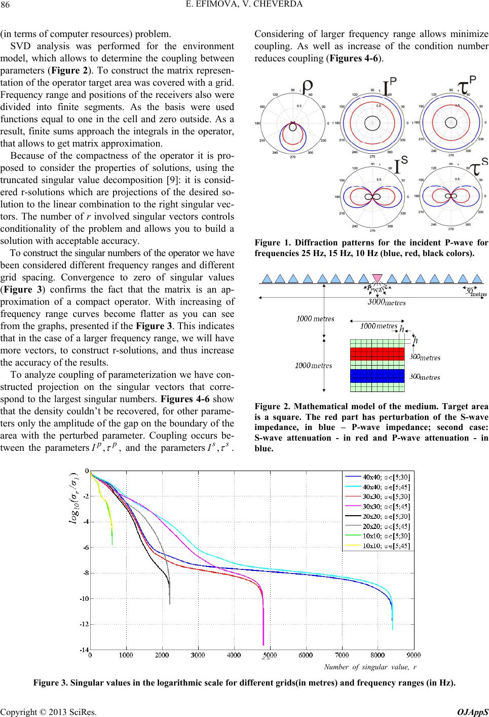
The scattering diagrams were constructed for the sets
of parameters:
1) Density, Lamé parameters, parameters of attenua-
tion ,,{,, }
p
s

;
2) Density, velocities, parameters of attenuation
{,, },,
p
sps
VV

;
3) Density, impedances, parameters of attenuation
{},,,,
p
sps
II

.
The best results were obtained for parameterization
{},,,,
p
sps
II

.
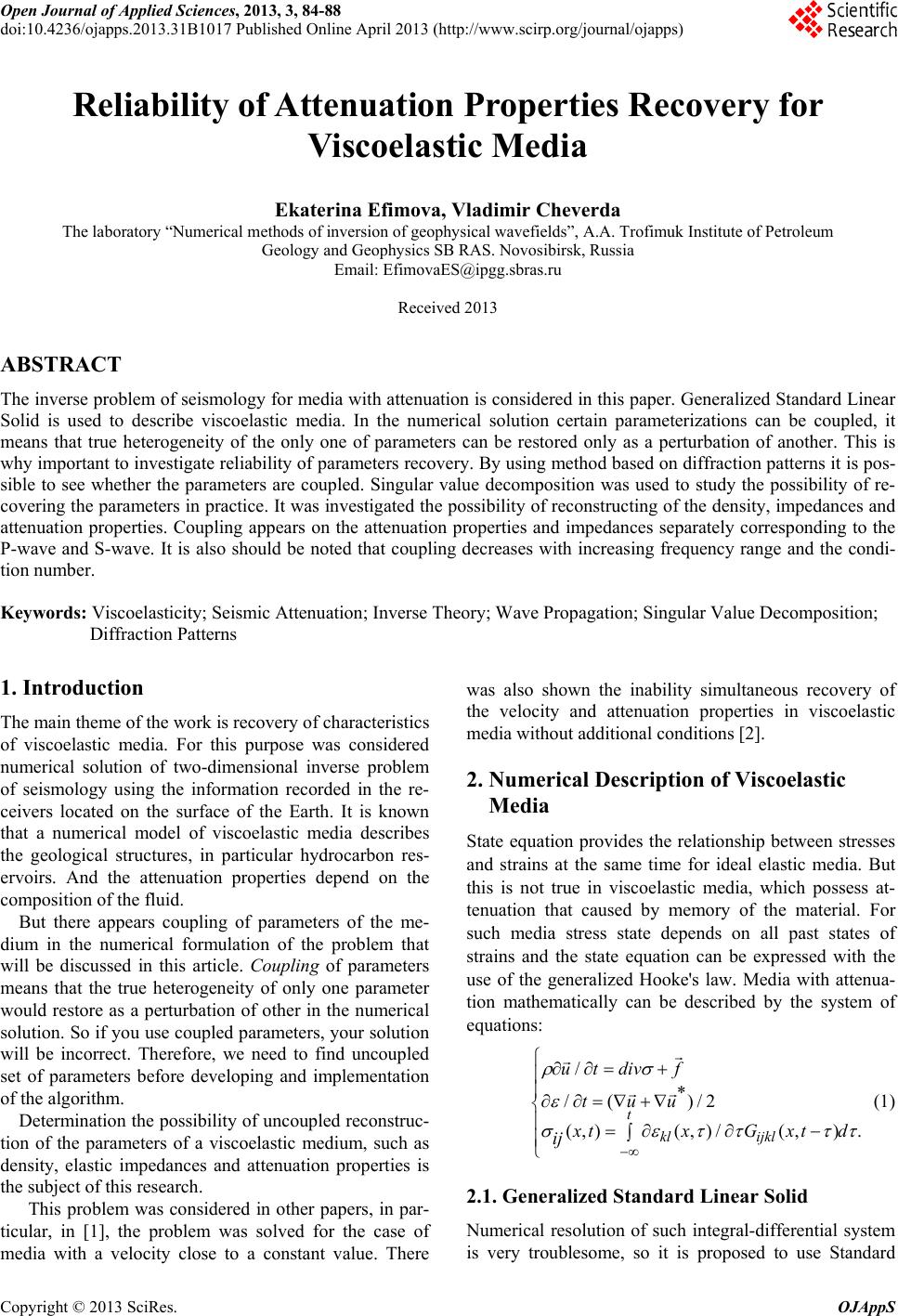
On Figure 1 are presented diffraction patterns for
parameterization {,,,, }
p
sps
II

in the case of inci-
dent P-wave and reflected P-,S-wawes. Diffraction pat-
terns for the parameters of attenuation and impedances
corresponding to P-or S-wave are similar in shape, that
indicates their coupling. Coupling may decrease when
considering frequency range, as there is different de-
pendence amplitude of the frequency for various pa-
rameters (Figure 1).
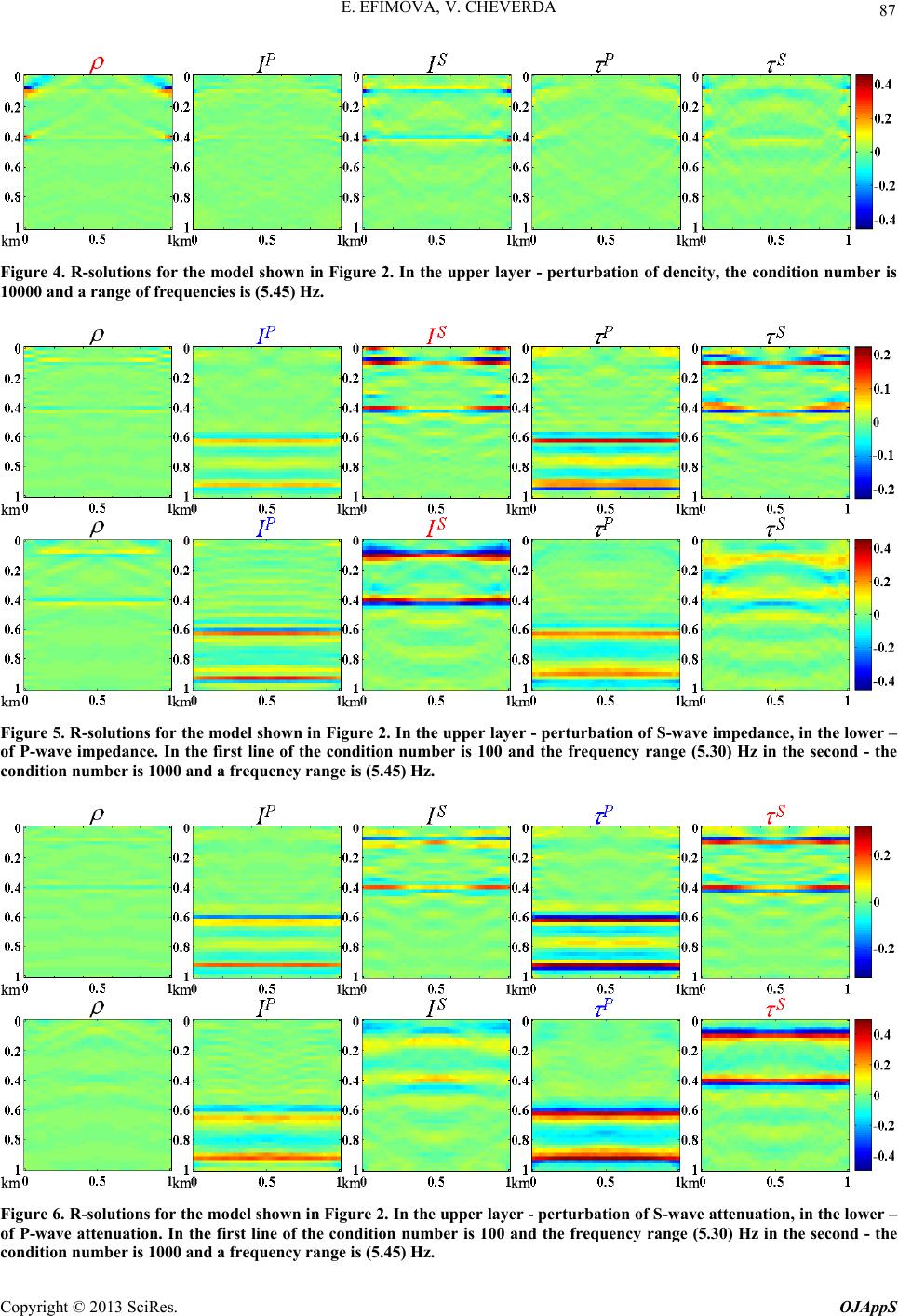
3.2. Singular Value Decomposition
To study the coupling and the possibility of recovery
parameters is also used a method based on singular value
decomposition (SVD) of a compact operator of the prob-
lem. Computation of singular value decomposition for an
arbitrary environment is very complicated and expensive
Copyright © 2013 SciRes. OJAppS
E. EFIMOVA, V. CHEVERDA
Copyright © 2013 SciRes. OJAppS
86
(in terms of computer resources) problem. Considering of larger frequency range allows minimize
coupling. As well as increase of the condition number
reduces coupling (Figures 4-6).
SVD analysis was performed for the environment
model, which allows to determine the coupling between
parameters (Figure 2). To construct the matrix represen-
tation of the operator target area was covered with a grid.
Frequency range and positions of the receivers also were
divided into finite segments. As the basis were used
functions equal to one in the cell and zero outside. As a
result, finite sums approach the integrals in the operator,
that allows to get matrix approximation.
Because of the compactness of the operator it is pro-
posed to consider the properties of solutions, using the
truncated singular value decomposition [9]: it is consid-
ered r-solutions which are projections of the desired so-
lution to the linear combin ation to th e right sing ular vec-
tors. The number of r involved singular vectors controls
conditionality of the problem and allows you to build a
solution with acceptable accuracy. Figure 1. Diffraction patterns for the incident P-wave for
frequencies 25 Hz, 15 Hz, 10 Hz (blue, red, black c o lor s).
To construct the singular numbers of the operator we have
been considered different frequency ranges and different
grid spacing. Convergence to zero of singular values
(Figure 3) confirms the fact that the matrix is an ap-
proximation of a compact operator. With increasing of
frequency range curves become flatter as you can see
from the graphs, presented if the Figure 3. This indicates
that in the case of a larger frequency range, we will have
more vectors, to construct r-solutions, and thus increase
the accuracy of the results.
To analyze coupling of parameterization we have con-
structed projection on the singular vectors that corre-
spond to the largest singular numbers. Figures 4-6 show
that the density couldn’t be recovered, for other parame-
ters only the amplitude of the gap on th e boundary of the
area with the perturbed parameter. Coupling occurs be-
tween the parameters,
p
p
I
, and the parameters,
s
s
I
.
Figure 2. Mathematical model of the medium. Target area
is a square. The red part has perturbation of the S-wave
impedance, in blue – P-wave impedance; second case:
S-wave attenuation - in red and P-wave attenuation - in
blue.
Number of singular value, r
Figure 3. Singular values in the logarithmic scale for different grids(in metres) and frequency ranges (in Hz).
E. EFIMOVA, V. CHEVERDA 87
Figure 4. R-solutions for the model shown in Figure 2. In the upper layer - perturbation of dencity, the condition number is
10000 and a range of frequencies is (5.45) Hz.
Figure 5. R-solutions for the model shown in Figure 2. In the upper layer - perturbation of S-wave impedance, in the lower –
of P-wave impedance. In the first line of the condition number is 100 and the frequency range (5.30) Hz in the second - the
condition number is 1000 and a frequency range is (5.45) Hz.
Figure 6. R-solutions for the model shown in Figure 2. In the upper layer - perturbation of S-wave attenuation, in the lower –
of P-wave attenuation. In the first line of the condition number is 100 and the frequency range (5.30) Hz in the second - the
condition number is 1000 and a frequency range is (5.45) Hz.
Copyright © 2013 SciRes. OJAppS
E. EFIMOVA, V. CHEVERDA
Copyright © 2013 SciRes. OJAppS
88
Figure 7. The scaled trace recorded in the first receiver in Fig. 2. Assumed the presence of P-wave attenuation: Q = 200, 60,
40, 20, and also in the linearized case. Right picture is zoomed rectangle from the left picture.
The presented in Figure 7 seismogram tracks shows
that the graph for the linearized case with initial ap-
proximation acquisitions 0
0,0
ps

0
(the first ap-
proximation step of the viscoelastic medium) is most
similar to the graph for the quality factor Q = 200. This
indicates that even a linear formulation gives good results.
4. Conclusions
To study the linearized operator of the dynamic theory of
elasticity for the viscoelastic media were used methods
based on diffraction patterns [8] and on the SVD-analysis
[9]. The target area was chosen as a homogeneous me-
dium with two areas, each has perturbation of only one
parameter. This option provides an obvious determina-
tion of coupling o f parameterizat i o n .
Coupling between the elastic impedances and the
quality factors (corresponding to the P- and S-waves
separately) was found.
By using diffraction patterns and singular value de-
composition analysis was shown reducing coupling be-
tween parameters of viscoelastic medium in the case of
increasing of the frequency range. Also was shown reduc-
ing coupling between parameters in the case of increasing
of the condition number of the numerical problem.
It is concluded that the use of high-quality provides
simultaneous reconstruction of impedances and quality
factors. Study of an independent recovery of the parame-
ters of viscoelastic medium with use of poor-quality data
have planned for the future work.
REFERENCES
[1] J. M. Carcione, “Seismic Modeling in Viscoelastic Me-
dia,” Geophysics, Vol. 58, No. 1, 1993, pp. 110-120.
doi:10.1190/1.1443340
[2] W.A. Mulder and B. Hak “An Ambiguity in Attenuation
Scattering Imaging,” Geophysical Journal International,
Vol. 178, 2009, pp. 1614-1624.
doi:10.1111/j.1365-246X.2009.04253.x
[3] S. Asvadurov, L. Knizhnerman and J. Pabon, “Fi-
nite-Difference Modeling of Viscoelastic Materials with
Quality Factors of Arbitrary Magnitude,” Geophysics,
Vol. 69, No. 3, 2004, pp. 817-824.doi:10.1190/1.1759468
[4] W. I. Futterman, “Dispersive Body Waves,” Journal of
Geophysical Research, Vol. 67, No. 13, 1962. pp. 5279-
5291. doi:10.1029/JZ067i013p05279
[5] H. -P. Liu, D. L. Anderson, H. Kanamori, “Velocity Dis-
persion due to Anelasticity; Implications for Seismology
and Mantle Composition,” Geophysical Journal of Royal
Astronomical Society, Vol. 47, 1976, pp. 41-58.
doi:10.1111/j.1365-246X.1976.tb01261.x
[6] J. O. Blanch, J. O. A. Robertsson and W. W. Symes,
“Modeling of a Constant Q: Methodology and Algorithm
for an Efficient and Optimally Inexpensive Viscoelastic
Technique,” Geophysics, Vol. 60, No. 1, 1995, pp.
176-184. doi:10.1190/1.1443744
[7] F. Assous and F. Collino, “A Numerical Method for the
Explanation of Sensitivity: The Case of the Identification
of the 2D Stratified Elastic Medium,” Inverse Problems,
Vol. 6, No. 4, 1990, pp. 487–514.
doi:10.1088/0266-5611/6/4/003
[8] A. Tarantola, “A Strategy for Nonlinear Elastic Inversion
of Seismic Reflection Data,” Geophysics, Vol. 51, No. 10,
1986, pp. 1893–1903. doi:10.1190/1.1442046
[9] V. A. Cheverda, V.I. Kostin, “R-Pseudoinverses for
Compact Operators in Hilbert Spaces: Existence and Sta-
bility,” Journal of Inverse and Ill-Posed Problems, Vol. 3,
No. 2, 1995, pp. 131–148. doi:10.1515/jiip.1995.3.2.131