Open Journal of Applied Sciences, 2013, 3, 1-6
doi:10.4236/ojapps.2013.31B1001 Published Online April 2013 (http://www.scirp.org/journal/ojapps)
Changepoint Analysis by Modified Empirical Likelihood
Method in Two-phase Linear Regression Models
Hualing Zhao1, Hanfeng Chen2, Wei Ning2
1Department of Statistics , School of Science, Wuhan University of Technology, Wuhan, Hubei , P.R. of China
2Department of Mathematics and Statistics, Bowling Green State University, Bowling Green, Ohio , USA
Received 2013
ABSTRACT
A changepoint in statistical applications refers to an observational time point at which the structure pattern changes
during a somewhat long-term experimentation process. In many cases, the change point time and cause are documented
and it is reasonably straightforward to statistically adjust (homogenize) the series for the effects of the changepoint.
Sadly many changepoint times are und ocumented and the changepo int times themselves are the main purpose of study.
In this article, the changepoint analysis in two-phrase linear regression models is developed and discussed. Following
Liu and Qian (2010)'s idea in the segmented linear regressio n models, the modified empirical likeliho od ratio statistic i s
proposed to test if there exists a changepoint during the long-term experiment and observation. The modified empirical
likelihood ratio statistic is computation-friendly and its -value can be easily approximated based on the large sample
properties. The procedure is applied to the Old Faithful geyser eruption data in October 1980.
Keywords: Changepoint; Extreme-Value Distribution; Modified Empirical Likelihood Ratio; Segmented Linear
Regression
1. Introduction
In recent years increasing interest has been shown in change-
point analysis in two-phrase linear regression models. A
changepoint in statistical applications refers to an obser-
vational time point at which the structure pattern changes
during a somewhat long-term experimentation process.
In many cases, the change point time and cause is docu-
mented and it is reasonably straightforward to statisti-
cally adjust (homogenize) the series for the effects of the
changepoint. Sadly many changepoint times are un-
documented and the changepoint times themselves are
the main interest of study. For example, one of the most
important problems in economics is to d etermine as early
as possible the starting as well as ending time point of a
suspected ongoing recession. In the environmental sci-
ences, scientists are of great interest to understand when
the global warming started or the Earth's mean surface
temperature rise in the past decades should be explained
by the normal variability of the Earth's surface tempera-
ture over time. (Indeed the official position of the World
Natural Health Organization in regards to global warm-
ing is that there is no global warming and claims that
global warming is nothing more than just another hoax.
See their official website: http://www.wnho.net.)
The two-phrase linear regression model may be ex-
pressed as follows:
(1)
where p
i
x
R are covariates,

and

are p-di-
mensional regression parameters, is a putative
changepoint at which the liner regression model changes
from one phrase to another, and the
1kn
are assumed to be
independent and identically distributed unobservable
measurement errors. The main interest in the two-phrase
linear regression model is to determine whether such a
change of phrase occurs or not and if it does, when the
change happens during the experiment or observation. In
the special case of simple linear regression, the model (1)
is often called segmental linear regression model. As
remarked by Liu and Qian (2010), widespread applica-
tions of two-phrase linear regression model (1) have ap-
peared in diverse research areas. See, e.g., in environ-
mental sciences, Piegors ch and Bailer (1997), in medical
science, Simith and Cook (1980), in epidemiology Pastor
and Gullar (1998), in econometrics Fiteni (2004) and
Koul and Qian (2002) , just for a few.
As described above, with responses yi and covariates xi,
central to the problem is to determine whether there exists
a changepoint during the long-term experiment or obser-
vation. In terms of statistical inference, that is to test
0:H



versus 1:H

 

H. L. ZHAO ET AL.
2
Put

1,, , n
yy y



, 
,

  and .

1,, n



Let
where , .
Then the model(1) has the matrix expression:
(2)
Dong (2004) proposes an empirical likelihood-type
Wald statistic to infer the changepoint. More recently,
Liu and Qian (2010 ) proposes an interesting and compu-
tationally easy empirical likelihood detecting procedure
in the segmented linear regression model. In this paper,
their ideas are applied to the model (1) to present a modi-
fied empirical likelihood ratio statistic to test .
The article is organized as follows. The modified em-
pirical likelihood ratio test procedure and its computa-
tional issues are present and discussed in the next section.
The null distribution of the modified empirical likelihood
ratio test statistic is studied for large samples and the
results are put in the Appendix for interested readers. The
modified empirical likelihood method is applied to a
real-life data set for changepoint analysis in Section 3.
2. The Modified Empirical Likelihood
Method
Following Liu an d Qian (2010)'s ideas, the modified em-
pirical likelihood method for changepoint analysis in the
two-phrase linear regression mode(1) is described as fol-
lows: For each given k, estimate the regression parame-
ters by least-square methods for each segment, fit the
response at via the least-square estimate of the
regression parameters for the segment of counter-part,
and then construct the empirical likelihood ratio statistic
based the fitting residuals. In the notations introduced in
the last section, the least-square estimates for and
are
;
where and .
Define
(3)
for and
(4)
The modified empirical likelihood ratio statistic is
(5)
Recall that is the dimension of the covariates, so
equal to the number of regression parameters in each
phrase. Reject the null hypothesis and as-
sert that a changepoint occurs, whenever is signifi-
cantly large.
It should be noted that the residuals are not the
ordinary least-squares fitting residuals but the residuals
of fitting at with swapped least-square estimates
of the regression parameters. Motivation leading to the
modified empirical likelihood ratio statistics is that
if and only if , i.e. holds.
Through simulation studies, Liu and Qian (2010)
investigate whether has an asymptotic Gumbel
extreme value distribution under the null hypothesis. We
establish the null asymptotic theory of that is given
in the Appendix for interested readers. It is proved under
regular conditions that if the null hypothesis is
true, can be approximated by in probabil-
ity with an approximation error in size for some
constant , where
(6)
with
It is then shown that for any t,
where
and . Thus for any t,
(7)
The above formula indicates that the limiting ex-
treme-value distribution has a convergence rate of .
For this reason, the authors suggest to use the distribution
of under null hypothesis to approximate the p-
value of in applications. As the asymptotic null
distribution is free of any population distribution, one can
easily approximate the p-value of by Monte
Carlo methods through simulating the null distribution of
.
The main advantage of the modified empirical likeli-
hood testing procedure based on is its easiness of
computation. The package can be used to
compute
As many researchers remarked (Liu and Qian, 2010;
and , 1997), the statistic
is sensitive to outliers when k is too small or too close to
the sample size. and (1997) proposed
the trimmed idea to overcome the problem. Let
. Define
when it is assumed that as

H. L. ZHAO ET AL.
3
According the asymptotic null distribution discussed
in last section, the p-value with the observed
is approximately that is very close
to 0, leading to the assertion that there exists a change-
point during the 270 eruptions of the Old Faithful geyser
in October 1980.
we have
when and are chosen to be constant, .
Liu and Qian (2010) suggests to use and
. Such a choice clearly satisfies. Another popu-
lar choice is , ; see Perron and
Vogelsang (1992). In p ar ticu l ar, if for ,
and where is the greatest integer
less than or equal to x, by Corollary A.3.1 of
and
4. Acknowledgements
The research is partially funded by the Fundamental Re-
search Funds for the Central Universities (No. 2011-IV-
116).
REFERENCES
3. A Real-Life Example [1] M. Csorgo and L. Horvnth, “Limit Theorem in
Change-Point Analysi,” Wiley Series in Probability and
Statistics, John Wiley & Sons: New York, 1997.
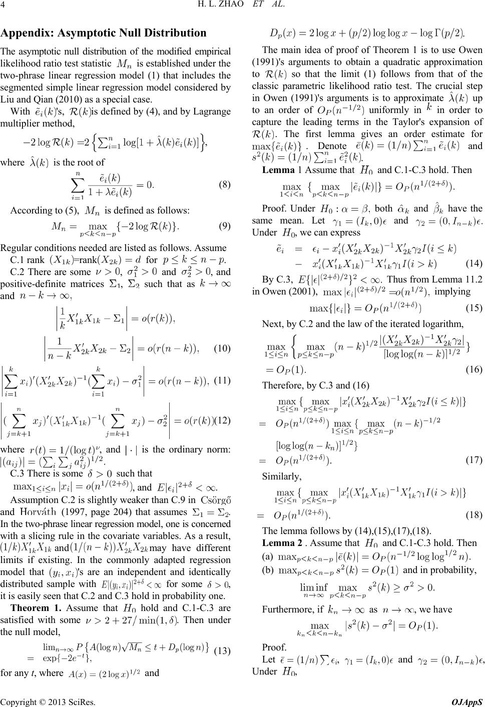
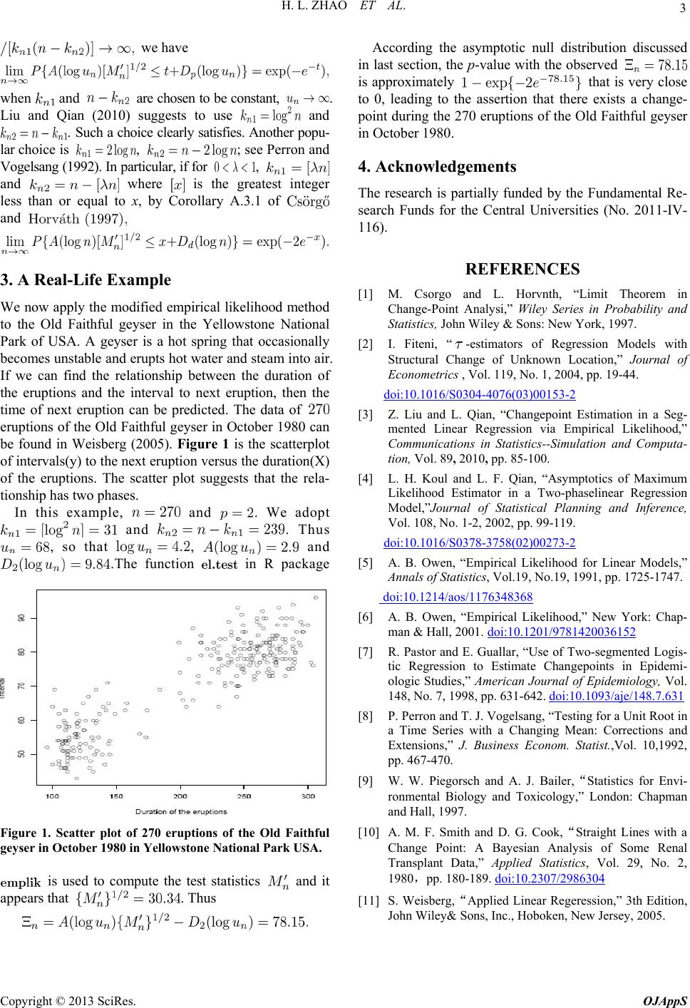
We now apply the modified empirical likelihood method
to the Old Faithful geyser in the Yellowstone National
Park of USA. A geyser is a hot spring that occasionally
becomes unstable and erupts hot water and steam into air.
If we can find the relationship between the duration of
the eruptions and the interval to next eruption, then the
time of next eruption can be predicted. The data of
eruptions of the Old Faithful geyser in October 1980 can
be found in Weisberg (2005). Figure 1 is the scatterplot
of intervals(y) to the next eruption versus the duration(X)
of the eruptions. The scatter plot suggests that the rela-
tionship has two phases.
[2] I. Fiteni, “-estimators of Regression Models with
Structural Change of Unknown Location,” Journal of
Econometrics , Vol. 119, No. 1, 2004, pp. 19-44.
doi:10.1016/S0304-4076(03)00153-2
[3] Z. Liu and L. Qian, “Changepoint Estimation in a Seg-
mented Linear Regression via Empirical Likelihood,”
Communications in Statistics--Simulation and Computa-
tion, Vol. 89, 2010, pp. 85-100.
[4] L. H. Koul and L. F. Qian, “Asymptotics of Maximum
Likelihood Estimator in a Two-phaselinear Regression
Model,”Journal of Statistical Planning and Inference,
Vol. 108, No. 1-2, 2002, pp. 99-119.
doi:10.1016/S0378-3758(02)00273-2
In this example, and . We adopt
and . Thus
, so that , and
.The function in R package [5] A. B. Owen, “Empirical Likelihood for Linear Models,”
Annals of Statistics, Vol.19, No.19, 1991, pp. 1725-1747.
doi:10.1214/aos/1176348368
[6] A. B. Owen, “Empirical Likelihood,” New York: Chap-
man & Hall, 2001. doi:10.1201/9781420036152
[7] R. Pastor and E. Guallar, “Use of Two-segmented Logis-
tic Regression to Estimate Changepoints in Epidemi-
ologic Studies,” American Journal of Epidemiology, Vol.
148, No. 7, 1998, pp. 631-642. doi:10.1093/aje/148.7.631
[8] P. Perron and T. J. Vogelsang, “Testing for a Unit Root in
a Time Series with a Changing Mean: Corrections and
Extensions,” J. Business Econom. Statist.,Vol. 10,1992,
pp. 467-470.
[9] W. W. Piegorsch and A. J. Bailer,“Statistics for Envi-
ronmental Biology and Toxicology,” London: Chapman
and Hall, 1997.
[10] A. M. F. Smith and D. G. Cook,“Straight Lines with a
Change Point: A Bayesian Analysis of Some Renal
Transplant Data,” Applied Statistics, Vol. 29, No. 2,
1980，pp. 180-189. doi:10.2307/2986304
Figure 1. Scatter plot of 270 eruptions of the Old Faithful
geyser in October 1980 in Yellowstone National Park USA.
is used to compute the test statistics and it
appears that . Thus [11] S. Weisberg,“Applied Linear Regeression,” 3th Edition,
John Wiley& Sons, Inc., Hoboken, New Jersey, 2005.

H. L. ZHAO ET AL.
4
Appendix: Asymptotic Null Distribution
The asymptotic null distribution of the modified empirical
likelihood ratio test statistic is established under the
two-phrase linear regression model (1) that includes the
segmented simple linear regression model considered by
Liu and Qian (2010) as a special case.
With 's, is defined by (4), and by Lagrange
multiplier method,
,
where is the root of
(8)
According to (5), is defined as follows:
(9)
Regular conditions needed are listed as follows. Assume
C.1 rank =rank for .
C.2 There are some , and , and
positive-definite matrices , such that as
and
(10)
(11)
(12)
where , and is the ordinary norm:
C.3 There is some such that
, and .
Assumption C.2 is slightly weaker than C.9 in
and (1997, page 204) that assumes .
In the two-phrase linear regression model, one is concerned
with a slicing rule in the covariate variables. As a result,
and may have different
limits if existing. In the commonly adapted regression
model that 's are an independent and identically
distributed sample with for some ,
it is easily seen that C.2 and C.3 hold in probability one.
Theorem 1. Assume that hold and C.1-C.3 are
satisfied with some . Then under
the null model,
(13)
for any t, where
.
The main idea of proof of Theorem 1 is to use Owen
(1991)'s arguments to obtain a quadratic approximation
to so that the limit (1) follows from that of the
classic parametric likelihood ratio test. The crucial step
in Owen (1991)'s arguments is to approximate up
to an order of uniformly in in r to
capture the leadin the Taylor's expansion of
orde
ing terms
. The first lemma gives an order estimate for
. Denote and
.
Lemma 1 Assume that and C.1-C.3 h old. Then
both and Proof. Under have the
sat me mean. Le an d
Under , we can express
(14)
By C.3, Thus from Lemm
in01), a 11.2 Owen (20 implying
)
Next, by C.2 and the law of the iterated
(15
logarithm,
(6)
Therefore,
1
by C.3 and (16)
(17)
Similarly,
(18)
The lemma follows by (14),(15),(17),(18).
Lemma 2 . Assume that
and
and C.1-C.3 hold. Then
(a)
and in probability, (b)
as , we have Furthermore, if
Proof.
Let , and ,
Under ,

H. L. ZHAO ET AL. 5
so that (25)and (26) become
(19)
By C.2 and the law of iterated logarithm,
Thus,
(20)
Similarly,
(21)
Combining (19),(20),(21), we have
The part (a) is proved.
Next consider . We may write
(22)
By C.2 and the law of iterated logarithm, we have
(23)
Similarly,
(24)
By C.2 and the the law of iterated logarithm again,
(25)
(26)
It is clear that for ,
(27)
(28)
The part (b) follows from(22-24),(27),(28). The pr
is complete. oof
Lemma 3. Assume that and C.1-C.3 hold. Then
for some
Proof. Since solves (8), similarly to Owen (2),
we consider 001
, So by Lemma 1, for some
(29)
By Lemma 2,
(30)
Therefore by (29),(30),
(31)
Now let By (31) and Lemma 1, it
follows that
Using Taylor expansion,
(32)
where , By Lemma
(31) 1 and
(33)
Therefore, by (31), Lemmas 1 and 2, we co
uniformly in k, nclude that
(34)

H. L. ZHAO ET AL.
6
The lemma follows from Lemma 2, (32) and (34),
with any
Proof of Theorem 1. First, we use Lemmas 1, 2 and 3
to obtain a quadratic approximation to ,
uniformly in .(38)
Combining (35),(36),(37),(38) yields that for any
Following Owen (2001, page 221)'
gu s ar- ments, denote . Using Taylor's expan-
sion,
,
(39)
Now applying Taylor expansion
(35)
,
where uniformly in k
as argue some d in (33). By Lemmas 1 and 3, for, we have for any
(40)
Denote i.e.,
Using the same arguments to the proof oorem
3.1.2 of f The and (1997), we have
(36)
Next by Lemma 3, for some
t
, for all Since
(37)
and
, it follows from
(40) that
The proof is complete.