 Journal of Water Resource and Protection, 2013, 5, 747-759 http://dx.doi.org/10.4236/jwarp.2013.57076 Published Online July 2013 (http://www.scirp.org/journal/jwarp) Agricultural Water Conservation in the High Plains Aquifer and Arikaree River Basin Adam Prior1, Ramchand Oad1, Kristoph-Dietrich Kinzli2 1Department of Civil and Environment Engineering, Colorado State University, Fort Collins, USA 2Department of Environmental and Civil Engineering, Florida Gulf Coast University, Fort Myers, USA Email: aprior@skybeam.com Received April 27, 2013; revised May 28, 2013; accepted June 19, 2013 Copyright © 2013 Adam Prior et al. This is an open access article distributed under the Creative Commons Attribution License, which permits unrestricted use, distribution, and reproduction in any medium, provided the original work is properly cited. ABSTRACT Yuma County is the top crop producing County in Colorado that is dependent on groundwater supplies from the High Plains aquifer for irrigation. The Arikaree River, a tributary of the Republican River in eastern Colorado, is supplied with water from the High Plains aquifer. The Arikaree River alluvium is also a habitat for many terrestrial invertebrates and the threatened Hybognathus hankinsoni (Brassy Minnow). The constant demand on the High Plains aquifer has created declining water levels at the linear rate of 0.183 m/year with the deepest pool in the Arikaree River drying up in 8 to 12 years. In addition to the demands for habitats, the surrounding irrigated agricultural lands require water for crop production. These challenges are currently confronting farmers in eastern Colorado and this research presents possible alternatives to meet these demands. This research presents a combination water balance model, water conservation model, and water conservation survey results from farmers in eastern Colorado to identify alternatives to extend the life of the Arikaree River. The first alternative was to examine the reduction in irrigation water from removing the 18 allu- vial irrigation wells that could extend the Arikaree River pools from drying up for 30 years. The other scenario found that water conservation practices with participation of 43%, 57%, and 62% of farmers would extend the drying time to 20, 30, and 40 years, respectively. The final alternative studied was the required participation in conservation practices to stop the decline of the High Plains Aquifer. The analysis found that 77% participation of farmers in all conservation alternatives or reducing pumping by 62.9% would be necessary to stabilize the High Plains Aquifer. Keywords: Agriculture; Conservation; Groundwater; Irrigation; Pumping; Water Balance 1. Introduction Throughout the United States, and especially in Colorado, farmers confront the challenges of meeting water needs for crop production, while trying to maintain natural ha- bitats and conserve dwindling water supplies. The Arika- ree River is a tributary of the Republican River on the Great Plains of Eastern Colorado and is groundwater dependent with flows from the underlying High Plains aquifer. The river is characterized by an extensive gallery of mature riparian cottonwoods (Populus deltoids), well- developed refuge habitat for threatened fish species such as the Brassy Minnow (Hybognathus hankinsoni), as well as habitat for many terrestrial invertebrates sus- tained by water from the High Plains aquifer. The ripar- ian habitat areas along the Arikaree River are a critical component of stream-riparian ecosystems in the Great Plains [1]. In addition to the demands for the mainte- nance of habitats, the surrounding irrigated agricultural land requires water as well. The irrigation water supply is groundwater pumped from the High Plains aquifer by high-capacity pumps. In recent years, the river has be- come a series of disconnected pools or has dried up en- tirely during the late summer. To sustain both a precari- ous regional agricultural economy and an aquatic/ripar- ian ecosystem, both dependent on groundwater for exis- tence, there must be tradeoffs to preserve this important resource. The research presented here provides practical guidelines for water conservation, water management practices, and identified feasible and realistic conserva- tion measures for farmers in Eastern Colorado. 1.1. Study Area The research study area was located in Yuma County, Colorado with the Yuma County border as the eastern and western boundaries. The north and south boundaries constitute the groundwater divide as shown in Figure 1 C opyright © 2013 SciRes. JWARP  A. PRIOR ET AL. 748 from geology and groundwater resources of Yuma Coun- ty, Colorado, USGS water-supply paper 1539-J [2]. The Arikaree River has headwaters on the plains in eastern Colorado that flow northeast through Kansas be- fore joining the Republican River in the southwest corner of Nebraska. The river is a fluctuating stream [4], pri- marily sustained by inflow from springs or seeps from the High Plains aquifer and by storm events. The average annual stream flow from 1932 to 2009 has decreased significantly as shown in Figure 2. After the introduction of groundwater pumping in the 1960’s, there is a marked decline in the average annual flows. The High Plains aquifer is a part of the Ogallala Aqui- fer, the largest aquifer in the United States. Colorado only has 4% of the High Plains aquifer available for us- able water [5,6]. Since the High Plains aquifer both feeds and connects to the Arikaree River, the geomorphology has a significant effect on flow regimes [7]. The Ogallala Figure 1. The Arikaree River basin within southern Yuma County [3]. Figure 2. Annual average stream flows in the Arikaree Ri- ver at Haigler, Nebraska from 1932 to 2009 [12]. Formation overlies the Pierre Shale and is made of layers of sand, gravel, clay, limestone, and sandstone [2]. Research has shown that the water table is declining by about 0.25 m/yr near the Arikaree River [8] with the average rate of decline of the water table at 0.34 m/yr [9]. Reference [10] determined an annual water table decline of 0.3 m in the High Plains. Data collected by the Colo- rado Division of Water Resources [11] found the average water table decline of 2.08 m from 1988 to 2002 that equaled a decline of 0.15 m per year. The Arikaree Groundwater Management District has reported a decline 1.14 m in saturated thickness from 1997 to 2004 or 0.16 m/year [13]. 1.2. Water Conservation Water conservation can be defined as long-term increase in the productive use of a water supply without compro- mising the desired water services. Water conservation in terms of agricultural production can also mean more effi- cient water use, transmission and distribution system effi- ciency improvements, reduced evaporation and runoff, and the production of crops with reduced water require- ments. Opportunities to address the concurrent water needs of irrigators and the stream flow requirements for fish habitat are many and diverse. A comprehensive lit- erature review was completed about the conservation methods and practices used throughout the country and in the arid western United States under conditions similar to the High Plains aquifer and Arikaree River alluvium. The water conservation alternatives were divided into five different categories that included field conservation practices, irrigation conservation practices, management conservation practices, water conservation programs, and lower consumptive use crop selection. Field practices for water conservation increase the amount of water stored in the soil profile by trapping or holding rain where it falls, or where there is some small movement as surface runoff [14]. Local farmers in a wa- ter conservation survey identified the no-tillage field practice as the most feasible conservation measure with approximately 20% of the corn acres in produced in the United States utilizing no-tillage practices. No-till field management can save 10.2 to 12.7 cm of water for corn in Kansas with the combined growing and non-growing season [15]. In eastern Colorado from 2000 to 2004, corn crop residue also showed to have a signifi- cant effect during the non-growing season (October to April) by increasing stored soil water by 5.08 cm when compared to conventional stubble mulch [16]. Wheat stu- bble will increase soil water storage by 5.08 to 6.35 cm when compared to bare soil [17]. Wheat straw and no-till corn stover will save 6.35 to 7.62 cm of water from early June to the end of the growing season [18]. In Akron, Colorado, it was determined that no-till with wheat resi- Copyright © 2013 SciRes. JWARP  A. PRIOR ET AL. 749 due accumulated 11.68 cm of recharge over the fall, win- ter, and spring compared to conventionally tilled wheat residue that only had 6.35 cm of recharge for a total sav- ings of 5.33 cm during the non-growing season [16]. Irrigated agriculture uses approximately 80% of all the available water supplies in the Western United States [19-22]. Center pivot sprinkler irrigation systems are the most common form of irrigation used in the High Plains of Colorado [22]. About 90% of the irrigation systems use center pivots and pump from the High Plains aquifer [23,24]. The development of multi-functional systems such as low energy precision application (LEPA) allow farmers to apply water and also practice precision appli- cation of herbicides, pesticides, and fertigation [25]. The LEPA systems are highly efficient and can achieve ap- plication efficiencies in the 95% to 98% range [26] and [27] while other research suggests efficiency ranges from 80% to 95% depending on management [22]. A common water saving upgrade of center pivots is to reduce operating pressure and apply water within or be- low the crop canopy. Upgrading sprinkler systems to low pressure heads with drop tubes reduces evaporation from the plant surface, especially for corn [28]. If properly uti- lized, these improvements can result in water savings of 10% to 15% compared to traditional center pivot sprink- ler applications [22]. In eastern Colorado, the climate is semi-arid requiring some level of irrigation during drought years to maxi- mize certain crop yields. Water conservation survey re- sults of eastern Colorado farmers found that drought tol- erant crops were the most preferred and feasible water conservation alternative. Today’s best drought-tolerant crop hybrids, developed through conventional breeding, often yield within 75% to 80% of their average low- stress yields under drought stress. Other research com- paring hybrid yields for the last three decades showed that genetic improvements have increased yields 2.6% per year [29] due to hybrid water stress tolerance [30]. Reference [31] discovered a new corn hybrid that stress- sed at 50% of crop required ET produced 27% higher yields, but with adequate water, both hybrids produced similar yields. Corn breeders have found a new germ- plasm that can reduce water usage by 10% [32]. Xu and Lascano [33] found new corn hybrids that produce the same silage yield with a 75% crop water requirement (CWR) [32]. A wide range of programs to conserve water through state and national agencies exist in Colorado, in Yuma County, and in the Arikaree River basin. The 2007 Cen- sus of Agriculture in Yuma County Profile [23] said that 432 farms out of the 970 total farms in Yuma County par- ticipated in agricultural conservation programs. The farm participation in conservation programs increased from 28% in 2002 to 45% in 2007 [23]. Water conservation survey results of eastern Colorado farmers found that water use limits were considered a feasible water con- servation alternative. Reference [34] conducted research over a 10-year period showing that applying 15.2 cm per crop using limited irrigation can achieve winter wheat yields at 99%, corn yields at 86%, and soybean at 88% of the full irrigation yields. With proper management of 25% - 50% water application reductions, the income re- duces by only 10% - 20% [34]. Another successful water use limit program by the Nebraska Upper Republican Natural Resources District (URNRD) allows 184.2 cm (36.8 cm/ year) of water in any five-year period [35]. The water use limits have required farmers to be more re- sourceful and creative in managing water allocations. Re- search from 1986 to 1999 demonstrated that, if required, farmers could survive with less water usage because they were only using 80% of the allocated water for the five- year period. Low consumptive use crops can be cool season crops that are subject to lower atmospheric demand that direct- ly relates to lower ET rates. Switching to crops with shorter growing seasons will reduce crop water and irri- gation demands in order to conserve water. This research has identified lower water use crops as any crop that has a lower consumptive use than corn, because corn is the dominant irrigated crop grown in eastern Colorado. 2. Materials and Methods 2.1. Water Balance To address water shortages and impacts to the Arikaree River, a water balance model was developed to compare pre-development (before pumping), post-development (after pumping), future conditions, and the possible im- pacts of water conservation. This water balance does not account for spatial and temporal variability in parameters such as recharge, evapotranspiration, and pumping, but provides the initial analysis in understanding and model- ing the aquifer and river hydrologic system. The model was broken into three distinctive model areas that include the regional High Plains aquifer, the alluvium model, and a complete model combining the High Plains aquifer and alluvium. Figures 3 and 4 show the pre- and post-deve- lopment model parameters used in the High Plains aqui- fer and alluvial aquifer with their respective data sources. Stream inflow from the aquifer was assumed to be 10% of the average stream flow data measured at USGS gauging station #6821360 (Haigler, NE) from 1933 to 1960 based on previous research done by Squires [8]. Stream outflow was the average stream flow measured at USGS gauging station #6821360 (Haigler, NE). The con- stant flux boundaries specified at the upstream boundary and at the downstream boundary of the alluvium estima- tions came from the 1958 head contour map [2]. The hy- Copyright © 2013 SciRes. JWARP  A. PRIOR ET AL. 750 Ralluv = 1.88 × 10⁷ m3 ETR = 8.10 × 10 ETG = 2.77 × 10 6 m3 7 m3 SFin = 2.30 × 10⁶ m3 (Qalluv)out = 1.03 × 10⁶ 3 SFout =2.30 × Alluvium Area = 28,530 ha Δ Storage ≈ 0 Qflux = 3.43 × 10⁷ m3 (Qalluv)in = 4.45 × 10⁶ 3 RHPA = 3.73 × 10⁷ m3 Ralluv = 1.88 × 10⁷ m3 Rtotal = 5.61 × 10⁷ m3 ETR = 8.10 × 10 ETG = 2.77 × 1 ETtotal = 3.58 × 6 m3 07 m3 107 m3 (Qtotal)in = 8.23 × 10⁶ m3 SFin = 2.30 × 10⁶ m3 Avg Q flux = 2.02 × 10 7 m 3 (1968-2010) R HPA = 3.73 × 10 7 m 3 (Qtotal)out = 7.80 × 10⁶ SFout = 2.30 × 10⁷m3 Regi onal Aqu ifer Area = 149,980 ha Δ Storage ≈ 0 RHPA = 3.73 × 10⁷ 3 Qflux = 3.43 × 10⁷ m3 (QHPA)in = 3.77 × 10⁶ (QHPA)out = 6.77 × 10⁶ m3 High Plains Aquifer Area = 121,450 ha Δ Storage ≈ 0 Figure 3. Initial water balance for the regional aquifer, High Plains aquifer, and the alluvial aquifer (terms in Bold solved in the pre-development water balance). draulic conductivities used in the groundwater bounda- ries and flows between hydraulic units were found by [36] with the alluvium hydraulic conductivities being three times higher than in the surrounding areas [2,36]. Ripar- ian evapotranspiration research by [37] established an average value of 89.2 cm in the 2006 growing season. This riparian evapotranspiration value affected an area of 909 ha as delineated by [3]. The alluvium grass evapo- transpiration was a calibration constant used to balance the alluvial water balance. The alluvium grass evapo- transpiration was assumed to be 10 cm/yr over the re- mainder of alluvium (27621.5 ha). Reference [38] found in Akron, Colorado that native grasses used 9 cm, 10.6 cm, and 19 cm respectively in 1966, 1966, and 1967. The alluvium grass evapotranspiration area was the remaining area in the alluvium outside the riparian area for a total area of 27,621 ha (28,530 ha - 909 ha). Recharge to the alluvium was determined to be approximately 15% from research completed by [39] and the regional water bal- ances [8]. For the alluvial aquifer, the estimation of the (Q HPA ) in = 3.77 × 10 6 High Plains Aquifer Area = 121,450 ha Δ Storage =−4.15 cm/yr (Q HPA ) out = 6.77 × 10 6 3 3 (Q w ) HPA = 6.45 × 10 7 m 3 R alluv = 1.88 × 10 7 m 3 ET R = 8.10 × 10 6 m 3 Alluvium Area = 28,530 ha Δ Storage = −2.43 cm/yr Avg Δy = −0.043 m/yr (average from 1968-2010) (Q alluv ) out = 1.03 × 10 6 m 3 (Q alluv ) in = 4.45 × 10 6 3 SF out = 7.65 × 10 6 m 3 (Ave) SF in = 7.65 × 10 5 m 3 (Q w ) alluv = 6.68 × 10 6 m 3 Avg Q flux = 2.02 × 10 7 m 3 (average from 1968-2010) Figure 4. Post-development water balance for the High Plains aquifer and the alluvial aquifer (terms in bold Solved for in post-development the water balance). uniform recharge was to be 6.6 cm, 15% of the average precipitation of 44 cm based on a lysimeter in the allu- vium along the South Platte in Fort Morgan County, Colorado [8,39]. Recharge to the High Plains aquifer was determined to be approximately 7% of the average pre- cipitation of 44 cm from 1932 to 1960 from research by [40,41]. The specified constant flux boundaries at the upstream boundary and at the downstream boundary of the High Plains aquifer estimates came from the 1958 head con- tour map [2]. Since the stream flow gauging station is approximately 11,300 meters downstream of the Yuma County boundary, the water balance did not use all of the groundwater flow leaving the boundary. The [2] contours shows the groundwater entering the river prior to the gauging station so they were not used in calculations to avoid double counting water flows. The groundwater flux out of the High Plains aquifer and into the alluvial aqui- fer was estimated from the pre-development calibrated regional models to match well data and to balance each region. A pre-development (1933-1960) water balance model was created to determine model calibration groundwater flux between the model boundaries Figure 3. The pre- development water balance has negligible storage change over time (ΔS = 0) for prior to 1960 [8]. A second water Copyright © 2013 SciRes. JWARP 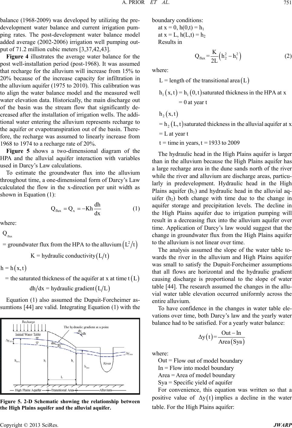 A. PRIOR ET AL. 751 balance (1968-2009) was developed by utilizing the pre- development water balance and current irrigation pum- ping rates. The post-development water balance model added average (2002-2006) irrigation well pumping out- put of 71.2 million cubic meters [3,37,42,43]. Figure 4 illustrates the average water balance for the post well-installation period (post-1968). It was assumed that recharge for the alluvium will increase from 15% to 20% because of the increase capacity for infiltration in the alluvium aquifer (1975 to 2010). This calibration was to align the water balance model and the measured well water elevation data. Historically, the main discharge out of the basin was the stream flow that significantly de- creased after the installation of irrigation wells. The addi- tional water entering the alluvium represents recharge to the aquifer or evapotranspiration out of the basin. There- fore, the recharge was assumed to linearly increase from 1968 to 1974 to a recharge rate of 20%. Figure 5 shows a two-dimensional diagram of the HPA and the alluvial aquifer interaction with variables used in Darcy’s Law calculations. To estimate the groundwater flux into the alluvium throughout time, a one-dimensional form of Darcy’s Law calculated the flow in the x-direction per unit width as shown in Equation (1): flux QQ x dh Kh dx (1) where: 2 uvium Lt flux Q =groundwater flux from the HPA to the all t at time t L K=hydraulic conductivityL h=hx,t =the saturated thickness of the aquifer at x dhdx=hydraulic gradientLL Equation (1) also assumed the Dupuit-Forcheimer as- sumtions [44] are valid. Integrating Equation (1) with the Figure 5. 2-D Schematic showing the relationship between boundary conditions: at x = 0, h(0,t) = h1 at x = L, h(L,t) = h2 Results in 22 flux2 1 K Q=h h 2L (2) where: gth of the transitional areaL L = len 11 hx,t= h0,tsaturated thickness in the HPA at x =0 at year t 2 2 hx,t =hL,tsaturated thickness in the alluvial aquifer at x =L at year t t=time in years,t=1933 to 2009 The hydraulic head in the High Plains aquifer is larger th he water table to- w ence in the changes in water table ele- va an in the alluvium because the High Plains aquifer has a large recharge area in the dune sands north of the river while the river and alluvium are discharge areas, particu- larly in predevelopment. Hydraulic head in the High Plains aquifer (h1) and hydraulic head in the alluvial aq- uifer (h2) both change with time due to the change in aquifer storage and precipitation levels. The decline in the High Plains aquifer due to irrigation pumping will result in a decreasing flux into the alluvium aquifer over time. Application of Darcy’s law would suggest that the change in groundwater flux from the High Plains aquifer to the alluvium is not linear over time. The analysis assumed the slope of t ards the river in the alluvium and High Plains aquifer was small to satisfy the Dupuit-Forcheimer assumptions that all flows are horizontal and the hydraulic gradient causing discharge is proportional to the slope of water table [44]. The research assumed the changes in the allu- vial water table elevation occurred uniformly across the entire alluvium. To have confid tions over time, both Darcy’s law and the yearly water balance had to be satisfied. For a yearly water balance: Out In Δyt= Area Sya where: low out of model boundary was written so that a po Out = F In = Flow into model boundary Area = Area of model boundary Sya = Specific yield of aquifer For convenience, this equation sitive value of Δyt implies a decline in the water table. For the High Plains aquifer: the High Plains aquifer and the alluvial aquifer. Copyright © 2013 SciRes. JWARP 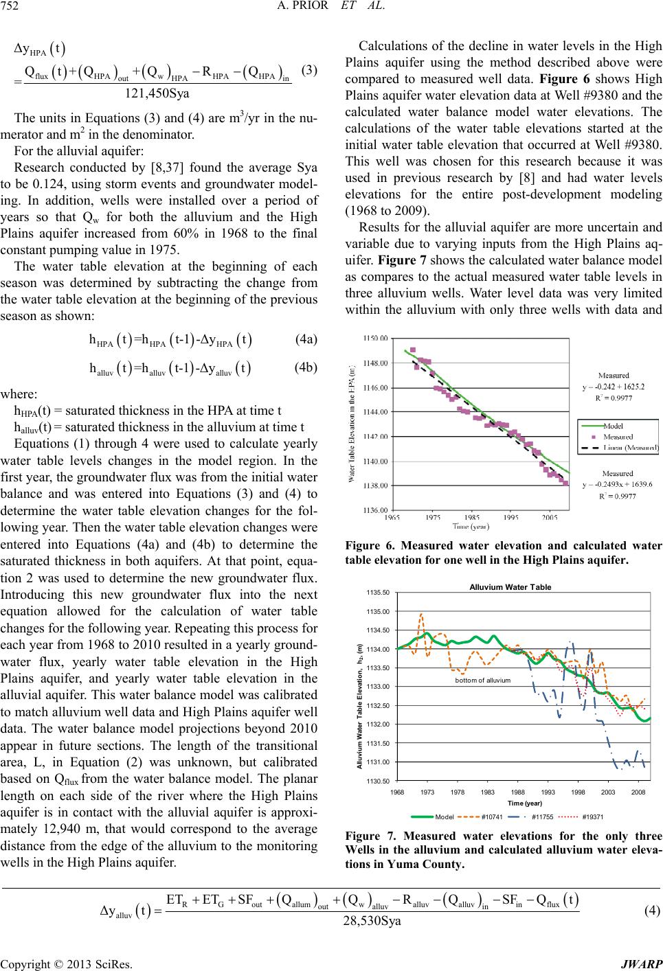 A. PRIOR ET AL. Copyright © 2013 SciRes. JWARP 752 Calculations of the decline in water levels in the High Plains aquifer using the method described above were compared to measured well data. Figure 6 shows High Plains aquifer water elevation data at Well #9380 and the calculated water balance model water elevations. The calculations of the water table elevations started at the initial water table elevation that occurred at Well #9380. This well was chosen for this research because it was used in previous research by [8] and had water levels elevations for the entire post-development modeling (1968 to 2009). HPA Δyt flux HPAwHPA HPA out in HPA Qt+Q+QR Q =121,450Sya (3) The units in Equations (3) and (4) are m3/yr in the nu- m d the average Sya to erator and m2 in the denominator. For the alluvial aquifer: 37] founResearch conducted by [8, be 0.124, using storm events and groundwater model- ing. In addition, wells were installed over a period of years so that Qw for both the alluvium and the High Plains aquifer increased from 60% in 1968 to the final constant pumping value in 1975. The water table elevation at the beginning of each se Results for the alluvial aquifer are more uncertain and variable due to varying inputs from the High Plains aq- uifer. Figure 7 shows the calculated water balance model as compares to the actual measured water table levels in three alluvium wells. Water level data was very limited within the alluvium with only three wells with data and ason was determined by subtracting the change from the water table elevation at the beginning of the previous season as shown: HPA t-1-Δyt (4a) HP h A HPA t=h alluv t-1-Δyt = saturated thickness in the HPA at time t e t y w alluvalluv ht=h where: (4b) hHPA(t) halluv(t) = saturated thickness in the alluvium at tim uEqations (1) through 4 were used to calculate yearl ater table levels changes in the model region. In the first year, the groundwater flux was from the initial water balance and was entered into Equations (3) and (4) to determine the water table elevation changes for the fol- lowing year. Then the water table elevation changes were entered into Equations (4a) and (4b) to determine the saturated thickness in both aquifers. At that point, equa- tion 2 was used to determine the new groundwater flux. Introducing this new groundwater flux into the next equation allowed for the calculation of water table changes for the following year. Repeating this process for each year from 1968 to 2010 resulted in a yearly ground- water flux, yearly water table elevation in the High Plains aquifer, and yearly water table elevation in the alluvial aquifer. This water balance model was calibrated to match alluvium well data and High Plains aquifer well data. The water balance model projections beyond 2010 appear in future sections. The length of the transitional area, L, in Equation (2) was unknown, but calibrated based on Qflux from the water balance model. The planar length on each side of the river where the High Plains aquifer is in contact with the alluvial aquifer is approxi- mately 12,940 m, that would correspond to the average distance from the edge of the alluvium to the monitoring wells in the High Plains aquifer. Figure 6. Measured water elevation and calculated water table elevation for one well in the High Plains aquifer. 1130.50 1131.00 1131.50 1132.00 1132.50 1133.00 1133.50 1134.00 1134.50 1135.00 1135.50 1968 1973 1978 1983 1988 1993 1998 2003 2008 Alluvium Wat er Table Elev at ion, h 2 , (m ) Time (year) lluv iu m W a te r Tab le Model 10741 11755 19371 bottom of alluvium Figure 7. Measured water elevations for the only three Wells in the alluvium and calculated alluvium water eleva- tions in Yuma County. RGoutallumwalluvalluvin flux out alluvin alluv ETET SFQQRQSFQt Δyt 28,530Sya (4) 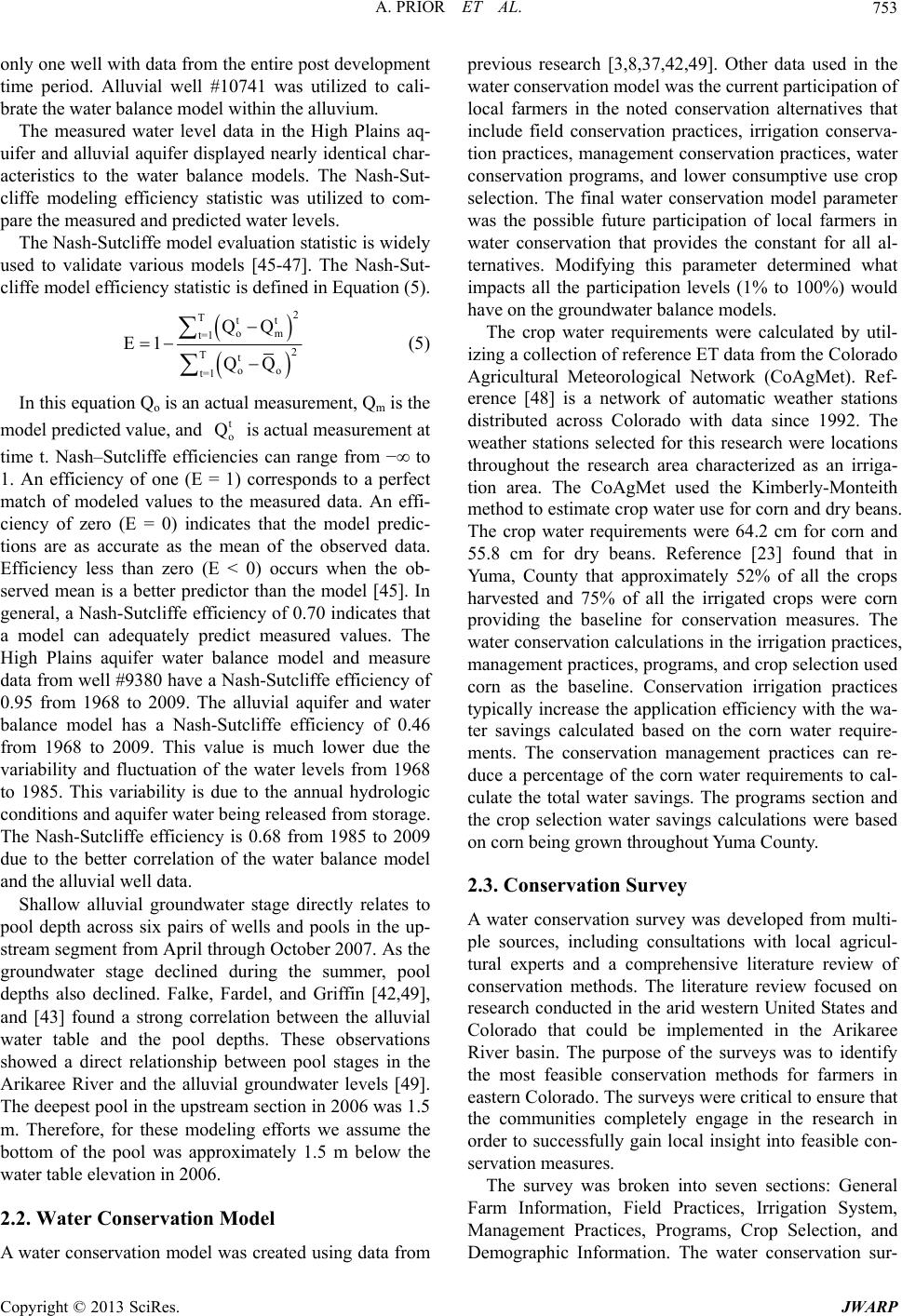 A. PRIOR ET AL. 753 only one well with data from the entire post development time period. Alluvial well #10741 was utilized to cali- brate the water balance model within the alluvium. The measured water level data in the High Plains aq- uifer and alluvial aquifer displayed nearly identical char- acteristics to the water balance models. The Nash-Sut- cliffe modeling efficiency statistic was utilized to com- pare the measured and predicted water levels. The Nash-Sutcliffe model evaluation statistic is widely used to validate various models [45-47]. The Nash-Sut- cliffe model efficiency statistic is defined in Equation (5). 2 Ttt om t=1 2 Tt QQ E1 QQ (5) oo t=1 In this equation Qo is an actual measu model predicteue, and t o Q is actual measurement at tim A water conservation model was created using data from previous research [3,8,37,42,49]. Other dat water conservation model was the current local farmers in the noted conservation alternatives that irrigation conserva- ion practices, water cused on western United States and emented in the Arikaree rement, Qm is the d val e t. Nash–Sutcliffe efficiencies can range from −∞ to 11. An efficiency of one (E = ) corresponds to a perfect match of modeled values toe measured data. An effi- th ciency of zero (E = 0) indicates that the model predic- tions are as accurate as the mean of the observed data. Efficiency less than zero (E < 0) occurs when the ob- served mean is a better predictor than the model [45]. In general, a Nash-Sutcliffe efficiency of 0.70 indicates that a model can adequately predict measured values. The High Plains aquifer water balance model and measure data from well #9380 have a Nash-Sutcliffe efficiency of 0.95 from 1968 to 2009. The alluvial aquifer and water balance model has a Nash-Sutcliffe efficiency of 0.46 from 1968 to 2009. This value is much lower due the variability and fluctuation of the water levels from 1968 to 1985. This variability is due to the annual hydrologic conditions and aquifer water being released from storage. The Nash-Sutcliffe efficiency is 0.68 from 1985 to 2009 due to the better correlation of the water balance model and the alluvial well data. Shallow alluvial groundwater stage directly relates to pool depth across six pairs of wells and pools in the up- stream segment from April through October 2007. As the groundwater stage declined during the summer, pool depths also declined. Falke, Fardel, and Griffin [42,49], and [43] found a strong correlation between the alluvial water table and the pool depths. These observations showed a direct relationship between pool stages in the Arikaree River and the alluvial groundwater levels [49]. The deepest pool in the upstream section in 2006 was 1.5 m. Therefore, for these modeling efforts we assume the bottom of the pool was approximately 1.5 m below the water table elevation in 2006. 2.2. Water Conservation Model a used in the participation of include field conservation practices, tion practices, management conservat conservation programs, and lower consumptive use crop selection. The final water conservation model parameter was the possible future participation of local farmers in water conservation that provides the constant for all al- ternatives. Modifying this parameter determined what impacts all the participation levels (1% to 100%) would have on the groundwater balance models. The crop water requirements were calculated by util- izing a collection of reference ET data from the Colorado Agricultural Meteorological Network (CoAgMet). Ref- erence [48] is a network of automatic weather stations distributed across Colorado with data since 1992. The weather stations selected for this research were locations throughout the research area characterized as an irriga- tion area. The CoAgMet used the Kimberly-Monteith method to estimate crop water use for corn and dry beans. The crop water requirements were 64.2 cm for corn and 55.8 cm for dry beans. Reference [23] found that in Yuma, County that approximately 52% of all the crops harvested and 75% of all the irrigated crops were corn providing the baseline for conservation measures. The water conservation calculations in the irrigation practices, management practices, programs, and crop selection used corn as the baseline. Conservation irrigation practices typically increase the application efficiency with the wa- ter savings calculated based on the corn water require- ments. The conservation management practices can re- duce a percentage of the corn water requirements to cal- culate the total water savings. The programs section and the crop selection water savings calculations were based on corn being grown throughout Yuma County. 2.3. Conservation Survey A water conservation survey was developed from multi- ple sources, including consultations with local agricul- tural experts and a comprehensive literature review of conservation methods. The literature review fo research conducted in the arid Colorado that could be impl River basin. The purpose of the surveys was to identify the most feasible conservation methods for farmers in eastern Colorado. The surveys were critical to ensure that the communities completely engage in the research in order to successfully gain local insight into feasible con- servation measures. The survey was broken into seven sections: General Farm Information, Field Practices, Irrigation System, Management Practices, Programs, Crop Selection, and Demographic Information. The water conservation sur- Copyright © 2013 SciRes. JWARP  A. PRIOR ET AL. 754 veys were distributed to 227 farmers in eastern Colorado, 41 surveys were returned for an 18% response rate. The top feasible conservation alternatives identified by local fa e from 1932 to 2009 of 0.44 m 1968 to 2009). The wa- odel of the High Plains aquifer estimated ecline was 0.242 m, which is similar to the y 1985, the alluvium water table es 87 to 20 gure 8). A possible re rmers include: no-tillage for the field practices; instal- lation of low-pressure sprinkler packages for irrigation systems; planting crops that use less water (i.e. drought tolerant crops) for the management practices; utilization of water limit incentive conservation programs; and planting lower water use crop such as dry beans to re- place the corn predominantly grown on approximately 52% of all croplands in Yuma County. These water con- servation survey results directed the water conservation analysis and water balance analysis on the High Plains aquifer and alluvial aquifer. The future water balance modeling utilized average or constant values for all parameters projected into the fu- ture. For example, the stream flow out was linearly de- creased at a rate of 12,007 m3/year for the best-fit line of the stream flow for the last 10 years. An average pa- rameter used in the future water balance modeling was the precipitation data averag eters. The actual future water levels in the High Plains aquifer fluctuated due to varying climatic conditions such as droughts and wet years. All future modeling projec- tions do not account for possible temporal climate change. The water levels of the High Plains aquifer and alluvial aquifer have significant impacts from recharge that are directly proportional to precipitation. Since large-scale agricultural irrigation began in Yuma County during the 1960s, the volume of groundwater used for irrigation has been relatively constant since 1975. In the [23] the irrigated land in Yuma County showed a de- crease of 0.7% from 2002 to 2007. The current irrigation pumping rates within the Arikaree River basin were as- sumed constant for forecasting. 3. Results The results for the High Plains aquifer are relatively straightforward, based on the measured data, and mod- eled information. The existing irrigation well water levels from this study indicate the High Plains aquifer is cur- rently declining at 0.249 m/year ( ter balance m groundwater d measured decline rate (Figure 6). Although a straight line can approximate the water table decline in the High Plains aquifer, the water table decline in the alluvium appears to be nonlinear. The existing alluvium well data suggest that from 1968 to approximately 1985 there was a slight decline in the alluvium water levels with fluctuations from climatic patterns (Figure 7). This could indicate the water in the alluvial aquifer was being released from the storage to supplement the lack of water from the High Plains aqui- fer flux. In approximatel tablished new declining water table equilibrium in cor- respondence to the declining High Plains aquifer. The goal of the modeling was to match the alluvial de- cline from 1985 to 2009. There were only 3 alluvial irri- gation wells with water table data and only one well (#10741) with data for the entire post-development mod- eling. The other two wells only had water table data from 1987 to 2009 (Figure 7). The well data for #19371 and #10741 have very similar linear declines from 19 09 so calibration of the model used these wells. The well data from #11755 is believed to be flashier due to the Pierre Shale geology located near the Colorado and Kansas bounder. The fluctuations of the alluvial water table directly related to the precipitation and stream flow in the Arikaree River Basin. This knowledge about the water table fluctuation leads to the conclusion that the alluvium has had a steady decline in water levels since 1985. The average decline of the alluvial water table from 1985 to 2009 was 0.079 m/year using data from wells #10741 and #19371. Falke [49] took a census of all refuge pool habitat within each of the three segments during late July, the period of lowest connectivity, from 2005-2007. No pools were present in the downstream segment during any of the surveys. In that time range, there were 172 to 218 pools identified in the upstream segment that contained water. The middle segment had between 27 to 35 pools surveyed for habitat [49]. Overall, the upstream segment contained significantly more fish habitat pools than the middle segment during the driest portion of 2005 to 2007 [49]. Given the higher incidence of drying in the downstream and middle segments [50], we chose to model only the upstream portion of the basin where the alluvial aquifer directly connects to the High Plains aquifer, and where essential habitats for fish are most likely to persist into the future. The first scenario examined the impacts of no changes to the current water usage and pumping rates throughout the High Plains aquifer and the alluvium. The High Plains aquifer will continue to decline at a linear rate of approximately 0.183 m/year (future projections). This rate is a lower decline rate than the measured rate of 0.249 m/year from 1968 to 2009 (Fi ason for this reduced decline is that the High Plains aquifer saturated thickness is decreasing and therefore the flow out of the High Plains aquifer is decreasing. The alluvial aquifer decline starts out slowly throughout the 1960’s and 1970’s and increases with time (1985 to 2009) because the alluvial aquifer is sensitive to changes in the groundwater flux (Figure 9). When less water feeds the alluvium, more water is taken from storage causing the water table elevation to decline. The modeling data matches well with water level data from well #10741. The change in groundwater flux from the High Plains Copyright © 2013 SciRes. JWARP 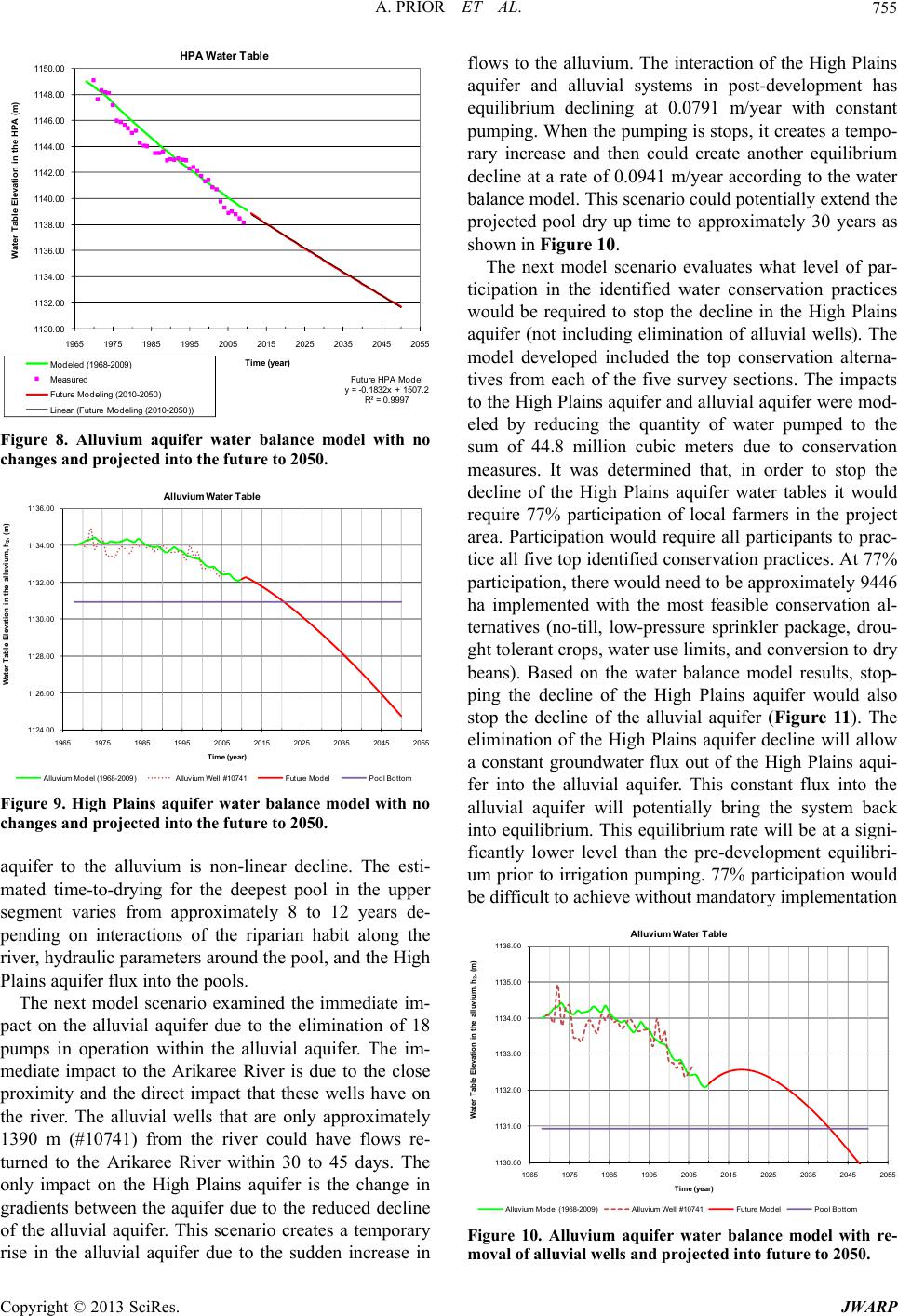 A. PRIOR ET AL. 755 1140. 0 0 1142. 0 0 1144. 0 0 1146. 0 0 1148. 0 0 1150. 0 0 e El evatio n in the HP A (m ) HPA Water Table Future HPA Model y = -0.1832x + 1507.2 R² = 0.9997 1965 1975 1985 1995 2005 2015 2025 2035 2045 2055 Water Tab l Time (y e ar ) 1130. 0 0 1132. 0 0 1134. 0 0 1136. 0 0 1138. 0 0 Modeled (1968-2009) Measured Future Modeli ng (2010-2050 ) Linear (F uture M o de ling (2010-205 0)) Figure 8. Alluvium aquifer water balance model with no changes and projected into the future to 2050. 1124.00 1126.00 1128.00 1130.00 1132.00 vation in the a 1134.00 1136.00 1965 1975 1985 1995 2005 2015 2025 2035 2045 2055 Water Table Elelluvium , h 2 , (m) Time (year) Alluvium Water Table Al l u v i u m M ode l 1968-2009 Alluvium Well #10741Future Model Pool Bot t o m Figure 9. High Plains aquifer water balance model with no changes and projected into the future to 2050. aquifer to the alluvium is non-linear decline. The esti- mated time-to-drying for the deepest pool in the upper segment varies from approximately 8 to 12 years de- pending on interactions of the riparian habit along the he next model scenario examined the immediate im- could have flows re- tu nd alluvial aquifer were mod- el river, hydraulic parameters around the pool, and the High Plains aquifer flux into the pools. T pact on the alluvial aquifer due to the elimination of 18 pumps in operation within the alluvial aquifer. The im- mediate impact to the Arikaree River is due to the close proximity and the direct impact that these wells have on the river. The alluvial wells that are only approximately 1390 m (#10741) from the river rned to the Arikaree River within 30 to 45 days. The only impact on the High Plains aquifer is the change in gradients between the aquifer due to the reduced decline of the alluvial aquifer. This scenario creates a temporary rise in the alluvial aquifer due to the sudden increase in flows to the alluvium. The interaction of the High Plains aquifer and alluvial systems in post-development has equilibrium declining at 0.0791 m/year with constant pumping. When the pumping is stops, it creates a tempo- rary increase and then could create another equilibrium decline at a rate of 0.0941 m/year according to the water balance model. This scenario could potentially extend the projected pool dry up time to approximately 30 years as shown in Figure 10. The next model scenario evaluates what level of par- ticipation in the identified water conservation practices would be required to stop the decline in the High Plains aquifer (not including elimination of alluvial wells). The model developed included the top conservation alterna- tives from each of the five survey sections. The impacts to the High Plains aquifer a ed by reducing the quantity of water pumped to the sum of 44.8 million cubic meters due to conservation measures. It was determined that, in order to stop the decline of the High Plains aquifer water tables it would require 77% participation of local farmers in the project area. Participation would require all participants to prac- tice all five top identified conservation practices. At 77% participation, there would need to be approximately 9446 ha implemented with the most feasible conservation al- ternatives (no-till, low-pressure sprinkler package, drou- ght tolerant crops, water use limits, and conversion to dry beans). Based on the water balance model results, stop- ping the decline of the High Plains aquifer would also stop the decline of the alluvial aquifer (Figure 11). The elimination of the High Plains aquifer decline will allow a constant groundwater flux out of the High Plains aqui- fer into the alluvial aquifer. This constant flux into the alluvial aquifer will potentially bring the system back into equilibrium. This equilibrium rate will be at a signi- ficantly lower level than the pre-development equilibri- um prior to irrigation pumping. 77% participation would be difficult to achieve without mandatory implementation 1133.00 1134.00 1135.00 1136.00 levati on i n the all uviu m, h 2 , (m) lluvium Water Table 1130.00 1131.00 1132.00 1965 1975 1985 1995 2005 2015 2025 2035 2045 2055 Water Tabl e E Time (year) lluvium Model 1968-2009 lluvium Well #10741Future Model Poo l Botto m Figure 10. Alluvium aquifer water balance model with re- moval of alluvial wells and projected into future to 2050. Copyright © 2013 SciRes. JWARP 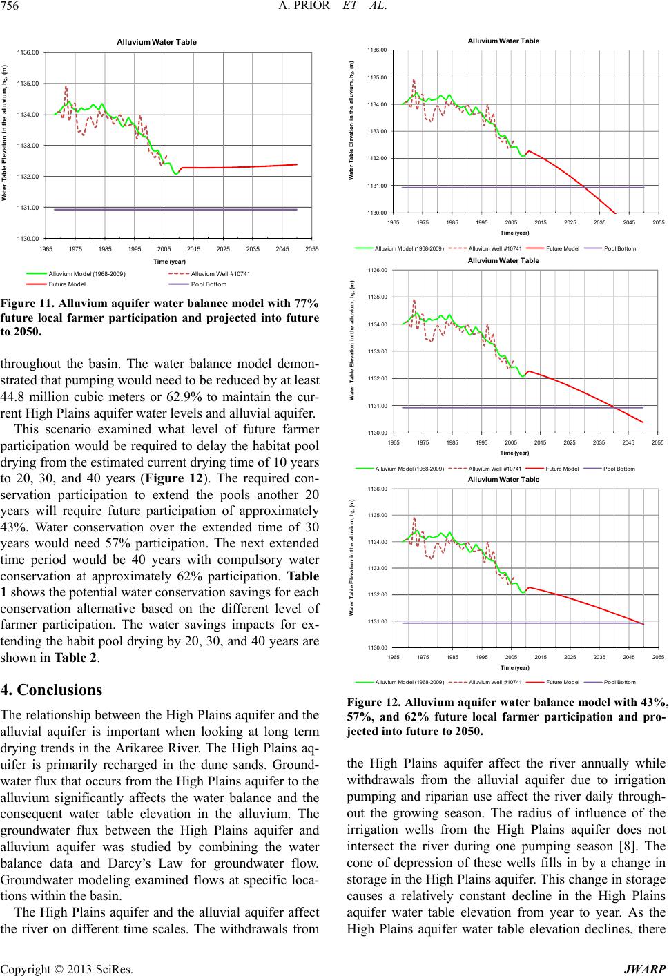 A. PRIOR ET AL. 756 1130.00 1131.00 1132.00 1133.00 1134.00 1135.00 1136.00 1965 1975 1985 1995 2005 2015 2025 Water Table Elevatio n in the all uvium , h 2 , (m) 203520452055 Alluvium Water Table Time (ye a r) Alluvium Model (1968-2009)Alluvium Well #10741 Future Model Pool Bottom Figure 11. Alluvium aquifer water balance model with 77% future local farmer participation and projected into future to 2050. throughout the basin. The water balance model demon- strated that pumping would need to be reduced by at least 44.8 million cubic meters or 62.9% to maintain the cur- rent High Plains aquifer water levels and alluvial aquifer. This scenario examined what level of future farmer participation would be required to delay the habitat pool drying from the estimated current drying time of 10 years to 20, 30, and 40 years (Figure 12). The required con- servation participation to extend the pools another 20 years will require future participation of approximately 43%. Water conservation over the extended time of 30 tion at approximately 62% participation. shows the potential water conservation savings for each uifer and the alluvial aquifer affect the river on different time scales. The withdrawals from years would need 57% participation. The next extended time period would be 40 years with compulsory water conserva Table 1 conservation alternative based on the different level of farmer participation. The water savings impacts for ex- tending the habit pool drying by 20, 30, and 40 years are shown in Table 2. 4. Conclusions The relationship between the High Plains aquifer and the alluvial aquifer is important when looking at long term drying trends in the Arikaree River. The High Plains aq- uifer is primarily recharged in the dune sands. Ground- water flux that occurs from the High Plains aquifer to the alluvium significantly affects the water balance and the consequent water table elevation in the alluvium. The groundwater flux between the High Plains aquifer and alluvium aquifer was studied by combining the water balance data and Darcy’s Law for groundwater flow. Groundwater modeling examined flows at specific loca- tions within the basin. The High Plains aq 1130.00 1131.00 1132.00 1133.00 1134.00 1135.00 1965 19751985 1995 2005 2015 20252035 2045205 1136.00 Water Table Elevation in the alluvi um, h 2 , (m) Time (year) lluvi um Wate r Tab le Alluvium Model (1968-2009)Alluvium Well # 10741Future Model Pool Bottom 1130.00 1131.00 1132.00 1133.00 1134.00 1135.00 1965 19751985 1995 20052015 20252035 2045 2055 Water Table Elevation in the alluvium, Time (ye ar) 1136.00 h 2 , (m) lluvium Water Table Alluvium Model (1968-2009)Alluvium Well #10741Future Model Pool Bottom 1130.00 1131.00 1132.00 1133.00 1134.00 1135.00 1136.00 1965 19751985 1995 20052015 2025 2035 20452055 Water Table Elevation in the alluvium, h 2 , (m) Time (yea r) Alluvium Water Table Alluvium Model (1968-2009)Alluvium Well #10741Future Model Pool B ott om Figure 12. Alluvium aquifer water balance model with 43%, 57%, and 62% future local farmer participation and pro- jected into future to 2050. the High Plains aquifer affect the river annually while withdrawals from the alluvial aquifer due to irrigation pumping and riparian use affect the river daily through- out the growing season. The radius of influence of the irrigation wells from the High Plains aquifer does not intersect the river during one pumping season [8]. The cone of depression of these wells fills in by a change in storage in the High Plains aquifer. This change in storage causes a relatively constant decline in the High Plains aquifer water table elevation from year to year. As the High Plains aquifer water table elevation declines, there Copyright © 2013 SciRes. JWARP 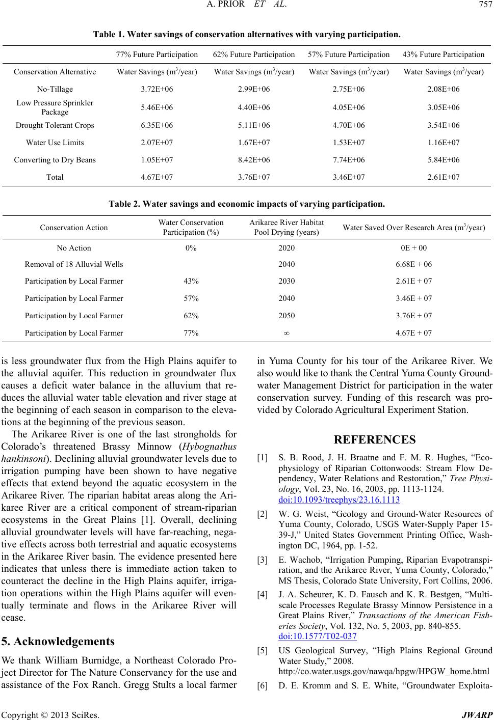 A. PRIOR ET AL. Copyright © 2013 SciRes. JWARP 757 Table 1. Water savings of conservation alicipation. 77% Future Participation 62% Future P ternatives with varying part articipation57% Future Participation 43% Future Participation Conservation Alternative Water Savings (m3/year) Water Savings (m3/year)Water Savings (m3/year) Water Savings (m3/year) No-Tillage 3.72E+06 2.99E Low Pressure Sprinkler Package 5.46E+06 4.40E Drought Tolerant Crops 6.35E+06 5.11E Water Use Limits 2.07E+07 1.67E Converting to Dry Beans 1.05E+07 8.42E Total 4.67E+07 76E +06 2.75E+06 2.08E+06 +06 4.05E+06 3.05E+06 +06 4.70E+06 3.54E+06 +07 1.53E+07 1.16E+07 +06 7.74E+06 5.84E+06 07 3.46E+07 2.61E+07 3.+ Table 2. Water savings and economic impacts of varying participation. Conservation Action ear Water Saved Over Research Area (m3/year) Water Conservation Arikaree River Habitat Participation (%) Pool Drying (ys) No Action 0% 2020 0E + 00 Removal of 18 Alluvial Wells 2040 6.68E + 06 Farmer 43% 2030 2.61E + 07 Participation by Local Farmer 57% 2040 3.46E + 07 mer 62% 2050 3.76E + 07 mer 77% ∞ 4.67E + 07 Participation by Local Participation by Local Far Participation by Local Far is less groter flux from theins aquifer to e alluvial aquifer. This reduction in groundwater flux deficit water ba duces the alluvial water table elevation and river stage at the beginn in compa- tions at the beginning of the previous seas The Arikarone of the last strlds for Colo Minnow (Hbognathus hanki oundwaterdue to irrigatio shown to hgative effec aquatic eco in the Arikaabitat areas athe Ari- karee River are a critical component of stream-riparian ecosy s [1]. Overeclining lluvial groundwater levels will have far-reaching, nega- River will ce uma County ur of the Arikaree River. We also would like to thank the Central Yuma County Ground- water conservation survey. Funding of this research was pro- o A REFERENCES [1] , J. H. Braatne and y of Riparian Cottoneam Flow De- ncy, Water Relations and,” Tree Physi- , Vol. 23, No. 16, 2003, pp. .1093/treephys/23.16.111 undwa High Pla in Y th causes a lance in the alluvium that re- water Management District for participation in the ning of each seasoavrison to the ele on. ee River is ongho rado’s threatened Brassyy nsoni). Declining alluvial gr n pumping have been levels ave ne ts that extend beyond thesystem ree River. The riparian hlong stems in the Great Plainall, d a tive effects across both terrestrial and aquatic ecosystems in the Arikaree River basin. The evidence presented here indicates that unless there is immediate action taken to counteract the decline in the High Plains aquifer, irriga- tion operations within the High Plains aquifer will even- tually terminate and flows in the Arikaree ase. 5. Acknowledgements We thank William Burnidge, a Northeast Colorado Pro- ject Director for The Nature Conservancy for the use and assistance of the Fox Ranch. Gregg Stults a local farmer for his to vided by Coloradgricultural Experiment Station. S. B. Rood physiolog F. M. R. Hughes, “Eco- woods: Str pende ology Restoration . 1113-1124 doi:10 3 [2] W. G. Weist, “Geology and Grr Resources of Yuma County, Colorado, USGS Water-Supply Paper 15- ound-Wate 39-J,” United States Government Printing Office, Wash- ington DC, 1964, pp. 1-52. [3] E. Wachob, “Irrigation Pumping, Riparian Evapotranspi- ration, and the Arikaree River, Yuma County, Colorado,” MS Thesis, Colorado State University, Fort Collins, 2006. [4] J. A. Scheurer, K. D. Fausch and K. R. Bestgen, “Multi- scale Processes Regulate Brassy Minnow Persistence in a Great Plains River,” Transactions of the American Fish- eries Society, Vol. 132, No. 5, 2003, pp. 840-855. doi:10.1577/T02-037 [5] US Geological Survey, “High Plains Regional Ground Water Study,” 2008. wqa/hpgw/HPGW_home.html hite, “Groundwater Exploita- http://co.water.usgs.gov/na [6] D. E. Kromm and S. E. W 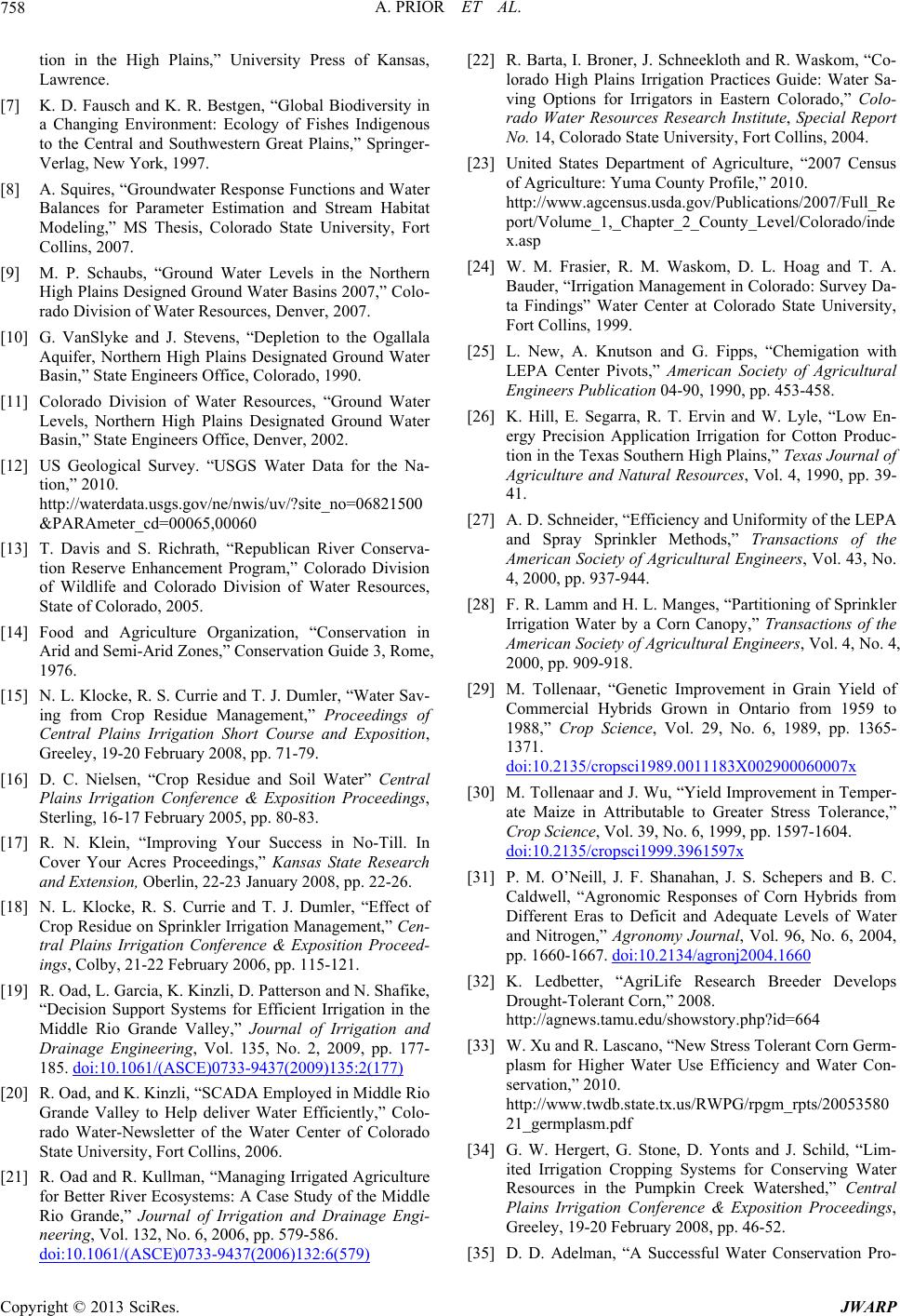 A. PRIOR ET AL. 758 tion in the High Plains,” University Press of Kansas, Lawrence. [7] K. D. Fausch and K. R. Bestgen, “Global Biodiversity in a Changing Environment: Ecology of Fishes Indigenous to the Central and Southwestern Great Plains,” Springer- Verlag, New York, 1997. [8] A. Squires, “Groundwater Response Functions and Water Balances for Parameter Estimation and Stream Habitat Modeling,” MS Thesis, Colorado State University, Fort Collins, 2007. [9] M. P. Schaubls in the Northern . GS Water Data for th e Organization, “Conservation in Your Success in No-Till. In n Sprinkler Irrigation Management,” Cen- 177) s, “Ground Water Leve High Plains Designed Ground Water Basins 2007,” Colo- rado Division of Water Resources, Denver, 2007. [10] G. VanSlyke and J. Stevens, “Depletion to the Ogallala Aquifer, Northern High Plains Designated Ground Water Basin,” State Engineers Office, Colorado, 1990 [11] Colorado Division of Water Resources, “Ground Water Levels, Northern High Plains Designated Ground Water Basin,” State Engineers Office, Denver, 2002. [12] US Geological Survey. “USe Na- tion,” 2010. http://waterdata.usgs.gov/ne/nwis/uv/?site_no=06821500 &PARAmeter_cd=00065,00060 [13] T. Davis and S. Richrath, “Republican River Conserva- tion Reserve Enhancement Program,” Colorado Division of Wildlife and Colorado Division of Water Resources, State of Colorado, 2005. [14] Food and Agricultur Arid and Semi-Arid Zones,” Conservation Guide 3, Rome, 1976. [15] N. L. Klocke, R. S. Currie and T. J. Dumler, “Water Sav- ing from Crop Residue Management,” Proceedings of Central Plains Irrigation Short Course and Exposition, Greeley, 19-20 February 2008, pp. 71-79. [16] D. C. Nielsen, “Crop Residue and Soil Water” Central Plains Irrigation Conference & Exposition Proceedings, Sterling, 16-17 February 2005, pp. 80-83. [17] R. N. Klein, “Improving Cover Your Acres Proceedings,” Kansas State Research and Extension, Oberlin, 22-23 January 2008, pp. 22-26. [18] N. L. Klocke, R. S. Currie and T. J. Dumler, “Effect of Crop Residue o tral Plains Irrigation Conference & Exposition Proceed- ings, Colby, 21-22 February 2006, pp. 115-121. [19] R. Oad, L. Garcia, K. Kinzli, D. Patterson and N. Shafike, “Decision Support Systems for Efficient Irrigation in the Middle Rio Grande Valley,” Journal of Irrigation and Drainage Engineering, Vol. 135, No. 2, 2009, pp. 177- 185. doi:10.1061/(ASCE)0733-9437(2009)135:2( Colorado on and Drainage [20] R. Oad, and K. Kinzli, “SCADA Employed in Middle Rio Grande Valley to Help deliver Water Efficiently,” Colo- rado Water-Newsletter of the Water Center of State University, Fort Collins, 2006. [21] R. Oad and R. Kullman, “Managing Irrigated Agriculture for Better River Ecosystems: A Case Study of the Middle Rio Grande,” Journal of IrrigatiEngi- neering, Vol. 132, No. 6, 2006, pp. 579-586. doi:10.1061/(ASCE)0733-9437(2006)132:6(579) [22] R. Barta, I. Broner, J. Schneekloth and R. Waskom, “Co- lorado High Plains Irrigation Practices Guide: Water Sa- h he Transactions of the 1959 to . 1365- ving Options for Irrigators in Eastern Colorado,” Colo- rado Water Resources Research Institute, Special Report No. 14, Colorado State University, Fort Collins, 2004. [23] United States Department of Agriculture, “2007 Census of Agriculture: Yuma County Profile,” 2010. http://www.agcensus.usda.gov/Publications/2007/Full_Re port/Volume_1,_Chapter_2_County_Level/Colorado/inde x.asp [24] W. M. Frasier, R. M. Waskom, D. L. Hoag and T. A. Bauder, “Irrigation Management in Colorado: Survey Da- ta Findings” Water Center at Colorado State University, Fort Collins, 1999. [25] L. New, A. Knutson and G. Fipps, “Chemigation wit LEPA Center Pivots,” American Society of Agricultural Engineers Publication 04-90, 1990, pp. 453-458. [26] K. Hill, E. Segarra, R. T. Ervin and W. Lyle, “Low En- ergy Precision Application Irrigation for Cotton Produc- tion in the Texas Southern High Plains,” Texas Journal of Agriculture and Natural Resources, Vol. 4, 1990, pp. 39- 41. [27] A. D. Schneider, “Efficiency and Uniformity of the LEPA and Spray Sprinkler Methods,” Transactions of t American Society of Agricultural Engineers, Vol. 43, No. 4, 2000, pp. 937-944. [28] F. R. Lamm and H. L. Manges, “Partitioning of Sprinkler Irrigation Water by a Corn Canopy,” American Society of Agricultural Engineers, Vol. 4, No. 4, 2000, pp. 909-918. [29] M. Tollenaar, “Genetic Improvement in Grain Yield of Commercial Hybrids Grown in Ontario from 1988,” Crop Science, Vol. 29, No. 6, 1989, pp 1371. doi:10.2135/cropsci1989.0011183X002900060007x [30] M. Tollenaar and J. Wu, “Yield Improvement in Temper- ate Maize in Attributable to Greater Stress Tolerance,” Crop Science, Vol. 39, No. 6, 1999, pp. 1597-1604. doi:10.2135/cropsci1999.3961597x [31] P. M. O’Neill, J. F. Shanahan, J. S. Schepers a Caldwell, “Agronomic Responses of Corn Hybrids from Different Eras to Deficit and Adequate Levels of Water and N nd B. C. itrogen,” Agronomy Journal, Vol. 96, No. 6, 2004, pp. 1660-1667. doi:10.2134/agronj2004.1660 [32] K. Ledbetter, “AgriLife Research Breeder Develops Drought-Tolerant Corn,” 2008. http://agnews.tamu.edu/showstory.php?id=664 urces in the Pumpkin Creek Watershed,” Central [33] W. Xu and R. Lascano, “New Stress Tolerant Corn Germ- plasm for Higher Water Use Efficiency and Water Con- servation,” 2010. http://www.twdb.state.tx.us/RWPG/rpgm_rpts/20053580 21_germplasm.pdf [34] G. W. Hergert, G. Stone, D. Yonts and J. Schild, “Lim- ited Irrigation Cropping Systems for Conserving Water Reso Plains Irrigation Conference & Exposition Proceedings, Greeley, 19-20 February 2008, pp. 46-52. [35] D. D. Adelman, “A Successful Water Conservation Pro- Copyright © 2013 SciRes. JWARP  A. PRIOR ET AL. Copyright © 2013 SciRes. JWARP 759 Region of Nebraska,” Journal of gram in a Semiarid American Water Resources Association, Vol. 39, No. 5, 2003, pp. 1079-1092. doi:10.1111/j.1752-1688.2003.tb03694.x [36] R. G. Borman, J. B. Linder, S. M. Bryn and J. Rutledge, Uni- and Akron, sources of ogeo R66-67DLR9,” Agricultural Engi- of Hydrology “The Ogallala Aquifer in the Northern High Plains of Colorado-Saturated Thickness in 1980; Saturated Thick- ness Changes, Predevelopment to 1980; Hydraulic Con- ductivity; Specific Yield; and Predevelopment and 1980 Probable Well Yields, Hydrologic Investigation A HA-671,” U.S. Geological Survey, 1983. tlas [37] L. Riley, “Finding the Balance: A Case Study of Irriga- tion, Riparian Evapotranspiration, and Hydrology of the Arikaree River Basin,” M.S. Thesis, Colorado State versity, Fort Collins, 2009. [38] R. J. Hanks, H. R. Gardner and R. L. Florian, “Evapo- transpiration-Climate Relations for Several Crops in the Central Great Plains,” Soil and Water Conservation Re- search Division, Agricultural Research Service, United States Department of Agriculture, Fort Collins 1968. [39] Willard Owens Consultants, “Ground Water Re the San Arroyo Creek Basin, Volume I Hydr logy, Computer Modeling, Conclusions and Recommenda- tions,” Prepared for Morgan County Quality Water Dis- trict, 1988. [40] D. L. Reddell, “Distribution of Groundwater Recharge Technical Report AE , neering Department, Colorado State University, Fort Col- lins, 1967, p. 132. [41] M. Sophocleous, “Groundwater Recharge Estimation and Regionalization: The Great Bend Prairie of Central Kan- sas and its Recharge Statistics,” Journal , Vol. 137, No. 1-4, 1992, pp. 113-140. doi:10.1016/0022-1694(92)90051-V [42] L. Fardal, “Effects of Groundwater Pumping for Irriga- tion on Stream Properties of the Arikaree River on the rado State University, Fort Collins, 2004. Colorado Plains,” M.S. Thesis, Colorado State University, Fort Collins, 2003. [43] S. Griffin, “Effect of Irrigation Practices on Stream De- pletion in the Arikaree River, Eastern Colorado,” M.S. Thesis, Colo [44] D. B. McWhorter and D. K. Sunada, “Ground-Water Hy- drology and Hydraulics,” Water Resources Publications, Highlands Ranch, Colorado, 1977. [45] R. H. McCuen, Z. Knight and A. G. Cutter, “Evaluation of the Nash-Sutcliffe Efficiency Index,” Journal of Hy- drologic Engineering, Vol. 11, No. 6, 2006, pp. 596-602. doi:10.1061/(ASCE)1084-0699(2006)11:6(597) [46] C. W. Downer and F. L. Ogden, “GSSHA: Model to Si- mulate Diverse Stream Flow Producing Processes,” Jour- nal Hydrologic Engineering, Vol. 9, No. 3, 2004, pp. 161-174. doi:10.1061/(ASCE)1084-0699(2004)9:3(161) [47] S. Birikundavyi, R. Labib, H. T. Trung and J. Rousselle, “Performance of Neural Networks in Daily Streamflow Forecasting,” Journal Hydrologic Engineering, Vol. 7, No. 5, 2002, pp. 392-398. doi:10.1061/(ASCE)1084-0699(2002)7:5(392) [48] Colorado Agricultural Meteorological Network, “About CoAgMet,” 2010. http://climate.colostate.edu/~coagmet/ [49] J. A. Falke, “Effects of Groundwater Withdrawal and Drought on Native Fishes and Their Habitats in the Ari- karee River, Colorado,” Ph.D. Thesis, Colorado State University, Fort Collins, 2009. [50] J. A. Scheurer, K. R. Bestgen and K. D. Fausch, “Resol- ving Taxonomy and Historic Distribution for Conserva- tion of Rare Great Plains Fishes: Hybognathus (Teleostei: Cyprinidae) in Eastern Colorado Basins,” Copeia, Vol. 1, 2003, pp. 1-12. doi:10.1643/0045-8511(2003)003[0001:RTAHDF]2.0.C O;2
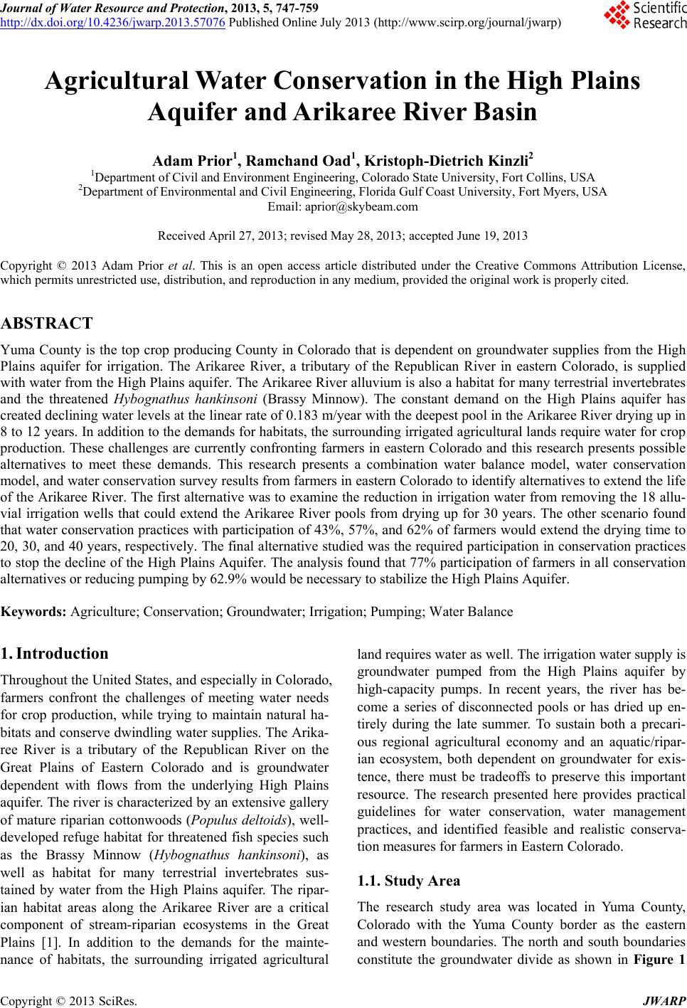
|