Configuration for Predicting Travel-Time Using Wavelet Packets and Support Vector Regression

doi:10.4236/jtts.2013.33023

Paper Menu >>

Journal Menu >>

Journal of Transportation Technologies, 2013, 3, 220-231

http://dx.doi.org/10.4236/jtts.2013.33023 Published Online July 2013 (http://www.scirp.org/journal/jtts)

Configuration for Predicting Travel-Time Using Wavelet

Packets and Support Vector Regression

Adeel Yusuf, Vijay K. Madisetti

School of Electrical and Computer Engineering, Georgia Institute of Technology, Atlanta, USA

Email: adeel@gatech.edu, vkm@gatech.edu

Received May 28, 2013; revised June 28, 2013; accepted July 5, 2013

tion License, which permits unrestricted use, distribution, and reproduction in any medium, provided the original work is properly

cited.

ABSTRACT

Travel-time prediction has gained significance over the years especially in urban areas due to increasing traffic conges-

tion. In this paper, the basic building blocks of the travel-time prediction models are discussed, with a small review of

the previous work. A model for the travel-time prediction on freeways based on wavelet packet decomposition and

support vector regression (WDSVR) is proposed, which used the multi-resolution and equivalent frequency distribution

ability of the wavelet transform to train the support vector machines. The results are compared against the classical

support vector regression (SVR) method. Our results indicated that the wavelet reconstructed coefficient when used as

an input to the support vector machine for regression performed better (with selected wavelets only), when compared

with the support vector regression model (without wavelet decomposition) with a prediction horizon of 45 minutes and

more. The data used in this paper was taken from the California Department of Transportation (Caltrans) of District 12

with a detector density of 2.73, experiencing daily peak hours except most weekends. The data was stored for a period

of 214 days accumulated over 5-minute intervals over a distance of 9.13 miles. The results indicated MAPE ranging

from 12.35% to 14.75% against the classical SVR method with MAPE ranging from 12.57% to 15.84% with a predic-

tion horizon of 45 minutes to 1 hour. The basic criteria for selection of wavelet basis for preprocessing the inputs of

support vector machines are also explored to filter the set of wavelet families for the WDSVR model. Finally, a con-

figuration of travel-time prediction on freeways is presented with interchangeable prediction methods.

Keywords: Travel-Time Prediction; Wavelet Packets; Support Vector Regression; Advanced Traveler Information

System

1. Introduction

Accurate travel-time forecast information has become a

fundamental component of all ATIS (Advanced Traffic

Information Systems). Currently, drivers demand an ac-

curate travel-time calculator that can forecast their com-

mute time in advance. This forecast is even more sig-

nificant in the morning and evening hours, when the

commuters face jammed freeways and they want to avoid

the peak-hour congestion. Drivers prefer precise infor-

mation of the future traffic conditions to manage their

route. Presently, most of the State Department traffic

websites provide the current traffic conditions, some sites

even calculate a forecast of the travel time based on the

historical data and/or current data by employing a suit-

able algorithm [1,2].

The travel-time is dependent on multiple factors that

are related through a complex-dependent relationship

with one another. Such factors include weather condi-

tions, driver behavior, and time of the day etc. This com-

plex-dependence makes the traffic data both non-linear

and non-stationary. Consequently, accurate prediction of

travel time becomes a challenging task.

Travel time prediction method can be classified from

different perspectives as shown in Figure 1. While, a

brief overview of all types is given in Section 2, the fo-

cus of this paper is on improving a short-term data driven

prediction method.

Table 1 shows a brief overview of the prior art in this

area. The prediction horizons in Table 1 range from 5

minutes to 60 minutes. However, lower forecast horizons

are not very useful for commuters in the real-world sce-

nario as there are delays involved in every module of the

travel-time prediction process; the process diagram of the

prediction process is shown in Figure 2.

Artificial Intelligence methods were extensively used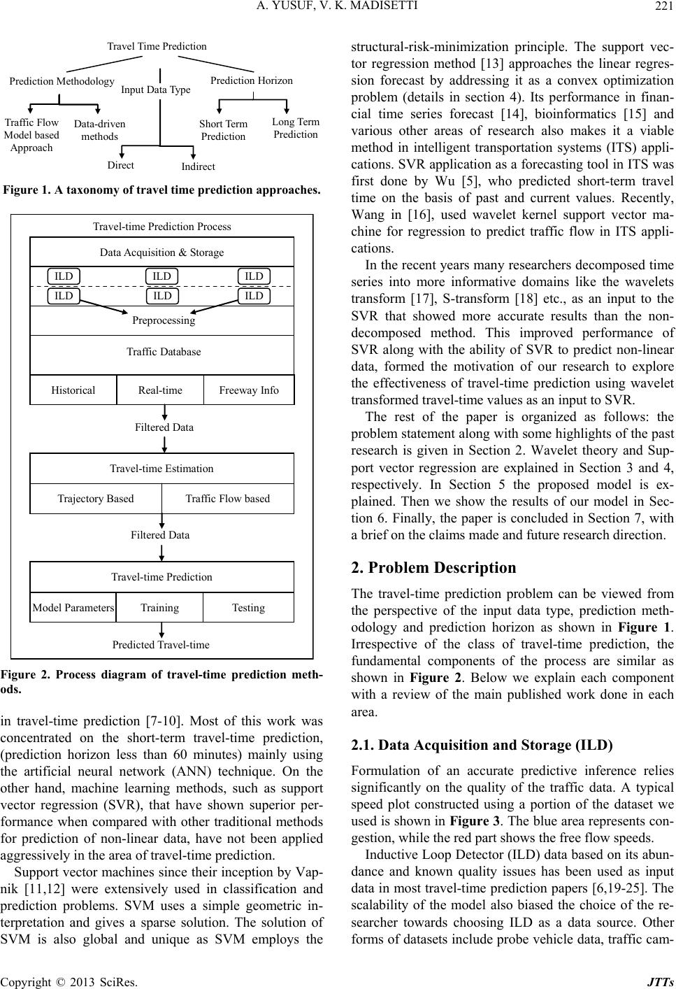

A. YUSUF, V. K. MADISETTI 221

Travel Time Prediction

Prediction Methodology Prediction Horizon

Short Term

Prediction

Long Term

Prediction

Data-driven

methods

Traffic Flow

Model based

Approach

Direct Indirect

Input Data Type

Figure 1. A taxonomy of travel time prediction approaches.

Data Acquisition & Storage

ILD

Preprocessing

Traffic Database

Historical Real-time Freeway Info

Filtered Data

Travel-time Estimation

Trajectory Based Traffic Flow based

Filtered Data

Travel-time Prediction

Model Parameters Testing

Training

Predicted Travel-time

Travel-time Prediction Process

Data Acquisition & Storage

ILD

Preprocessing

Traffic Database

Historical Real-time Freeway Info

Filtered Data

Travel-time Estimation

Trajectory Based Traffic Flow based

Filtered Data

Travel-time Prediction

Model Parameters Testing Training

Predicted Travel-time

Figure 2. Process diagram of travel-time prediction meth-

ods.

in travel-time prediction [7-10]. Most of this work was

concentrated on the short-term travel-time prediction,

(prediction horizon less than 60 minutes) mainly using

the artificial neural network (ANN) technique. On the

other hand, machine learning methods, such as support

vector regression (SVR), that have shown superior per-

formance when compared with other traditional methods

for prediction of non-linear data, have not been applied

aggressively in the area of travel-time prediction.

Support vector machines since their inception by Vap-

nik [11,12] were extensively used in classification and

prediction problems. SVM uses a simple geometric in-

terpretation and gives a sparse solution. The solution of

SVM is also global and unique as SVM employs the

structural-risk-minimization principle. The support vec-

tor regression method [13] approaches the linear regres-

sion forecast by addressing it as a convex optimization

problem (details in section 4). Its performance in finan-

cial time series forecast [14], bioinformatics [15] and

various other areas of research also makes it a viable

method in intelligent transportation systems (ITS) appli-

cations. SVR application as a forecasting tool in ITS was

first done by Wu [5], who predicted short-term travel

time on the basis of past and current values. Recently,

Wang in [16], used wavelet kernel support vector ma-

chine for regression to predict traffic flow in ITS appli-

cations.

In the recent years many researchers decomposed time

series into more informative domains like the wavelets

transform [17], S-transform [18] etc., as an input to the

SVR that showed more accurate results than the non-

decomposed method. This improved performance of

SVR along with the ability of SVR to predict non-linear

data, formed the motivation of our research to explore

the effectiveness of travel-time prediction using wavelet

transformed travel-time values as an input to SVR.

The rest of the paper is organized as follows: the

problem statement along with some highlights of the past

research is given in Section 2. Wavelet theory and Sup-

port vector regression are explained in Section 3 and 4,

respectively. In Section 5 the proposed model is ex-

plained. Then we show the results of our model in Sec-

tion 6. Finally, the paper is concluded in Section 7, with

a brief on the claims made and future research direction.

2. Problem Description

The travel-time prediction problem can be viewed from

the perspective of the input data type, prediction meth-

odology and prediction horizon as shown in Figure 1.

Irrespective of the class of travel-time prediction, the

fundamental components of the process are similar as

shown in Figure 2. Below we explain each component

with a review of the main published work done in each

area.

2.1. Data Acquisition and Storage (ILD)

Formulation of an accurate predictive inference relies

significantly on the quality of the traffic data. A typical

speed plot constructed using a portion of the dataset we

used is shown in Figure 3. The blue area represents con-

gestion, while the red part shows the free flow speeds.

Inductive Loop Detector (ILD) data based on its abun-

dance and known quality issues has been used as input

data in most travel-time prediction papers [6,19-25]. The

scalability of the model also biased the choice of the re-

searcher towards choosing ILD as a data source. Other

orms of datasets include probe vehicle data, traffic cam- f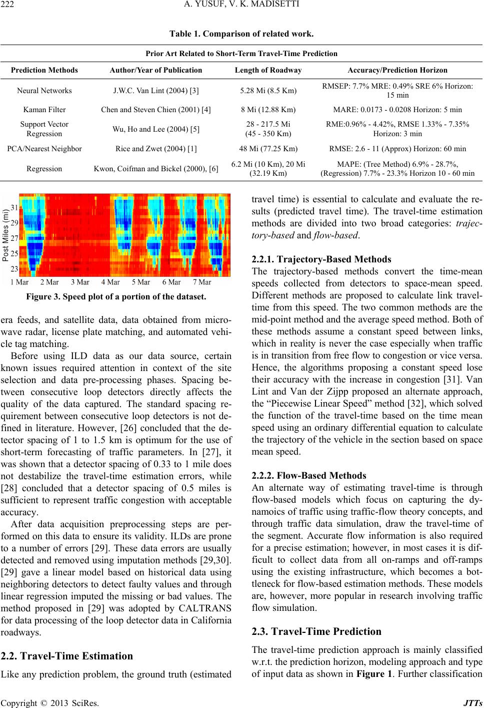

A. YUSUF, V. K. MADISETTI

222

Table 1. Comparison of related work.

Prior Art Related to Short-Term Travel-Time Prediction

Prediction Methods Author/Year of Publication Length of Roadway Accuracy/Prediction Horizon

Neural Networks J.W.C. Van Lint (2004) [3] 5.28 Mi (8.5 Km) RMSEP: 7.7% MRE: 0.49% SRE 6% Horizon:

15 min

Kaman Filter Chen and Steven Chien (2001) [4] 8 Mi (12.88 Km) MARE: 0.0173 - 0.0208 Horizon: 5 min

Support Vector

Regression Wu, Ho and Lee (2004) [5] 28 - 217.5 Mi

(45 - 350 Km)

RME:0.96% - 4.42%, RMSE 1.33% - 7.35%

Horizon: 3 min

PCA/Nearest Neighbor Rice and Zwet (2004) [1] 48 Mi (77.25 Km) RMSE: 2.6 - 11 (Approx) Horizon: 60 min

Regression Kwon, Coifman and Bickel (2000), [6] 6.2 Mi (10 Km), 20 Mi

(32.19 Km)

MAPE: (Tree Method) 6.9% - 28.7%,

(Regression) 7.7% - 23.3% Horizon 10 - 60 min

travel time) is essential to calculate and evaluate the re-

sults (predicted travel time). The travel-time estimation

methods are divided into two broad categories: trajec-

tory-based and flow-based.

Figure 3. Speed plot of a portion of the dataset.

era feeds, and satellite data, data obtained from micro-

wave radar, license plate matching, and automated vehi-

cle tag matching.

Before using ILD data as our data source, certain

known issues required attention in context of the site

selection and data pre-processing phases. Spacing be-

tween consecutive loop detectors directly affects the

quality of the data captured. The standard spacing re-

quirement between consecutive loop detectors is not de-

fined in literature. However, [26] concluded that the de-

tector spacing of 1 to 1.5 km is optimum for the use of

short-term forecasting of traffic parameters. In [27], it

was shown that a detector spacing of 0.33 to 1 mile does

not destabilize the travel-time estimation errors, while

[28] concluded that a detector spacing of 0.5 miles is

sufficient to represent traffic congestion with acceptable

accuracy.

After data acquisition preprocessing steps are per-

formed on this data to ensure its validity. ILDs are prone

to a number of errors [29]. These data errors are usually

detected and removed using imputation methods [29,30].

[29] gave a linear model based on historical data using

neighboring detectors to detect faulty values and through

linear regression imputed the missing or bad values. The

method proposed in [29] was adopted by CALTRANS

for data processing of the loop detector data in California

roadways.

2.2. Travel-Time Estimation

Like any prediction problem, the ground truth (estimated

2.2.1. Trajectory-Based Methods

vert the time-mean

2.2.2. Flow -Based Metho ds

g travel-time is through

2.3. Travel-Time Prediction

ch is mainly classified

The trajectory-based methods con

speeds collected from detectors to space-mean speed.

Different methods are proposed to calculate link travel-

time from this speed. The two common methods are the

mid-point method and the average speed method. Both of

these methods assume a constant speed between links,

which in reality is never the case especially when traffic

is in transition from free flow to congestion or vice versa.

Hence, the algorithms proposing a constant speed lose

their accuracy with the increase in congestion [31]. Van

Lint and Van der Zijpp proposed an alternate approach,

the “Piecewise Linear Speed” method [32], which solved

the function of the travel-time based on the time mean

speed using an ordinary differential equation to calculate

the trajectory of the vehicle in the section based on space

mean speed.

An alternate way of estimatin

flow-based models which focus on capturing the dy-

namoics of traffic using traffic-flow theory concepts, and

through traffic data simulation, draw the travel-time of

the segment. Accurate flow information is also required

for a precise estimation; however, in most cases it is dif-

ficult to collect data from all on-ramps and off-ramps

using the existing infrastructure, which becomes a bot-

tleneck for flow-based estimation methods. These models

are, however, more popular in research involving traffic

flow simulation.

The travel-time prediction approa

w.r.t. the prediction horizon, modeling approach and type

of input data as shown in Figure 1. Further classification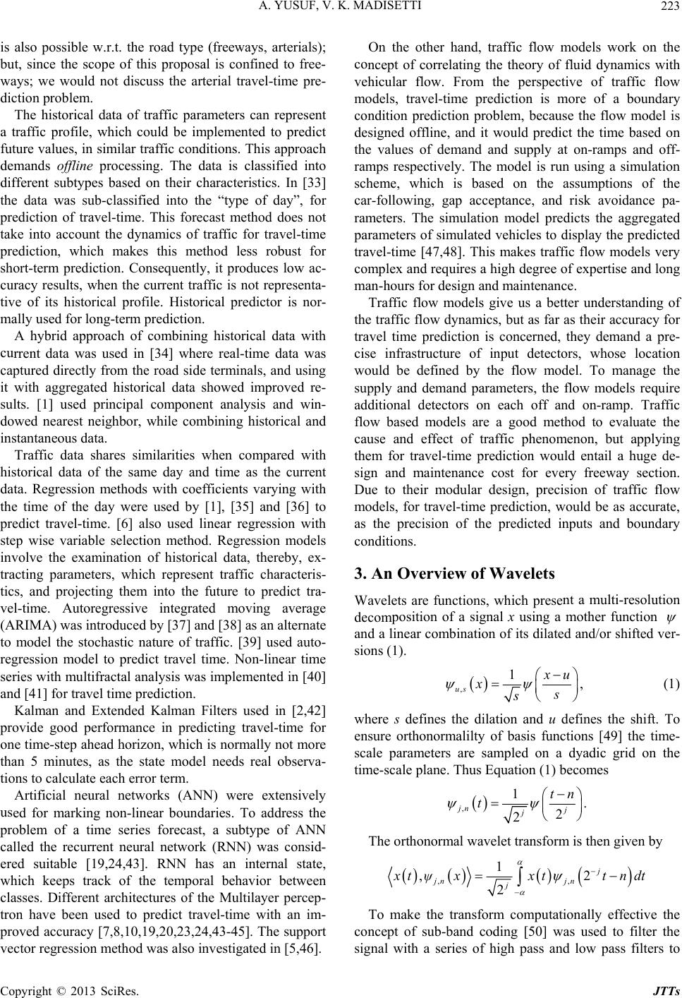

A. YUSUF, V. K. MADISETTI 223

is also possible w.r.t. the road type (freeways, arterials);

but, since the scope of this proposal is confined to free-

ways; we would not discuss the arterial travel-time pre-

diction problem.

The historical data of traffic parameters can represent

historical data with

es similarities when compared with

ilters used in [2,42]

N) were extensively

understanding of

3. An Overview of Wavelets

nt a multi-resolution

traffic profile, which could be implemented to predict

future values, in similar traffic conditions. This approach

demands offline processing. The data is classified into

different subtypes based on their characteristics. In [33]

the data was sub-classified into the “type of day”, for

prediction of travel-time. This forecast method does not

take into account the dynamics of traffic for travel-time

prediction, which makes this method less robust for

short-term prediction. Consequently, it produces low ac-

curacy results, when the current traffic is not representa-

tive of its historical profile. Historical predictor is nor-

mally used for long-term prediction.

A hybrid approach of combining

rrent data was used in [34] where real-time data was

captured directly from the road side terminals, and using

it with aggregated historical data showed improved re-

sults. [1] used principal component analysis and win-

dowed nearest neighbor, while combining historical and

instantaneous data.

Traffic data shar

storical data of the same day and time as the current

data. Regression methods with coefficients varying with

the time of the day were used by [1], [35] and [36] to

predict travel-time. [6] also used linear regression with

step wise variable selection method. Regression models

involve the examination of historical data, thereby, ex-

tracting parameters, which represent traffic characteris-

tics, and projecting them into the future to predict tra-

vel-time. Autoregressive integrated moving average

(ARIMA) was introduced by [37] and [38] as an alternate

to model the stochastic nature of traffic. [39] used auto-

regression model to predict travel time. Non-linear time

series with multifractal analysis was implemented in [40]

and [41] for travel time prediction.

Kalman and Extended Kalman F

ovide good performance in predicting travel-time for

one time-step ahead horizon, which is normally not more

than 5 minutes, as the state model needs real observa-

tions to calculate each error term.

Artificial neural networks (AN

ed for marking non-linear boundaries. To address the

problem of a time series forecast, a subtype of ANN

called the recurrent neural network (RNN) was consid-

ered suitable [19,24,43]. RNN has an internal state,

which keeps track of the temporal behavior between

classes. Different architectures of the Multilayer percep-

tron have been used to predict travel-time with an im-

proved accuracy [7,8,10,19,20,23,24,43-45]. The support

vector regression method was also investigated in [5,46].

On the other hand, traffic flow models work on the

ncept of correlating the theory of fluid dynamics with

vehicular flow. From the perspective of traffic flow

models, travel-time prediction is more of a boundary

condition prediction problem, because the flow model is

designed offline, and it would predict the time based on

the values of demand and supply at on-ramps and off-

ramps respectively. The model is run using a simulation

scheme, which is based on the assumptions of the

car-following, gap acceptance, and risk avoidance pa-

rameters. The simulation model predicts the aggregated

parameters of simulated vehicles to display the predicted

travel-time [47,48]. This makes traffic flow models very

complex and requires a high degree of expertise and long

man-hours for design and maintenance.

Traffic flow models give us a better

e traffic flow dynamics, but as far as their accuracy for

travel time prediction is concerned, they demand a pre-

cise infrastructure of input detectors, whose location

would be defined by the flow model. To manage the

supply and demand parameters, the flow models require

additional detectors on each off and on-ramp. Traffic

flow based models are a good method to evaluate the

cause and effect of traffic phenomenon, but applying

them for travel-time prediction would entail a huge de-

sign and maintenance cost for every freeway section.

Due to their modular design, precision of traffic flow

models, for travel-time prediction, would be as accurate,

as the precision of the predicted inputs and boundary

conditions.

Wavelets are functions, which prese

decomposition of a signal x using a mother function



and a linear combination of its dilated and/or shifted ve

sions (1).













us 

s (1)

where s defines the dilation and u defines the shift. To

ensure orthonormalilty of basis functions [49] the time-

scale parameters are sampled on a dyadic grid on the

time-scale plane. Thus Equation (1) becomes



1









jn j

The orthonormal wavelet transform is then given by

 















jjn n

xt ψ

xtt ndt

To make the transform computationally effective the

concept of sub-band coding [50] was used to filter the

signal with a series of high pass and low pass filters to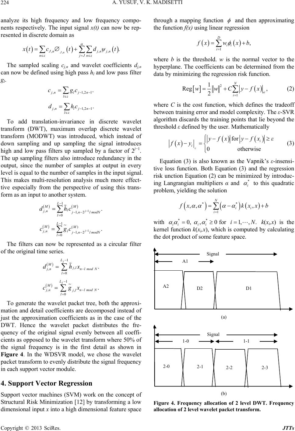

A. YUSUF, V. K. MADISETTI

224

analyze its high frequency and low frequency compo-

nents respectively. The input signal x(t) can now be rep-

resented in discrete domain as

 









Jnjn jn

nz jJnz

xtctd ψt.

The sampled scaling cj,n and wavelet coefficients dj,n

,21

To add translation-invariance in discrete wavelet

tra

n now be defined using high pass hl and low pass filter

gl.







jnl jn

cgc







jnl jn

dhc

nsform (DWT), maximum overlap discrete wavelet

transform (MODWT) was introduced, which instead of

down sampling and up sampling the signal introduces

high and low pass filters up sampled by a factor of 2j−1.

The up sampling filters also introduce redundancy in the

output, since the number of samples at output in every

level is equal to the number of samples in the input signal.

This makes multi-resolution analysis much more effect-

tive especially from the perspective of using this trans-

form as an input to another system.







1LM

,1, 2







j

nl modN

dhc





1()

,1, 2







j

jn jnl m

lodN

ccg

The filters can now be represented as a circular filter

of the original time series.













nnl

dhx

modN











nnl

cgx

modN

To generate the wavelet packet tree, both the approxi-

4. Support Vector Regression

on the concept of

ation and detail coefficients are decomposed instead of

just the approximation coefficients as in the case of the

DWT. Hence the wavelet packet distributes the fre-

quency of the original signal evenly between all coeffi-

cients as opposed to the wavelet transform where 50% of

the signal frequency is in the first detail as shown in

Figure 4. In the WDSVR model, we chose the wavelet

packet transform to evenly distribute the signal frequency

in each support vector module.

Support vector machines (SVM) work

Structural Risk Minimization [12] by transforming a low

dimensional input x into a high dimensional feature space

through a mapping function



and then approximating

the function f(x) using linear rression eg

 







ii

xwx

where b is the threshold. w is the normal vector to the

hyperplane. The coefficients can be determined from the

data by minimizing the regression risk function.





Reg ,









wwCyfx (2)

where C is the cost function, which defines the tradeoff

between training error and model complexity. The ε-SVR

algorithm discards the training points that lie beyond the

threshold ε defined by the user. Mathematically

 



for



0 otherwise





yfxyfx









fx y (3)

Equation (3) is also known as the Vapnik’s ε-insensi-

tive loss function. Both Equation (3) and the regression

risk unction Equation (2) can be minimized by introduc-

ing Langrangian multipliers α and *



i to this quadratic

problem, yielding the solution





,, ,

 





ii

xxb

with **

0, ,0

 





iii i

function k(xi,x), wh

for k(xi,x) is the

1,, .iN

putedkernel ich is com by calculating

the dot product of some feature space.

A2 D1

Signal

D2 D1

(a)

2-0 D22-1 2-32-2

1-0 1-1

Signal

(b)

Figure 4. Frequency allocatlevel DWT. Frequency

allocation of 2 level wavelet packet transform.

ion of 2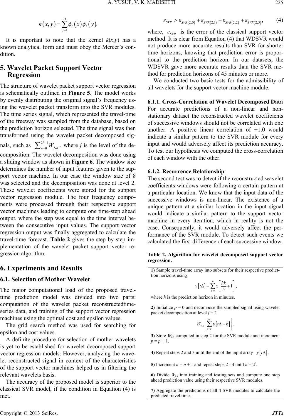

A. YUSUF, V. K. MADISETTI 225

 





kxyx y

1j

It is important to note that the kernel k(x,y) has a

known an

elet Packet Support Vector

or regression

alytical form and must obey the Mercer’s con-

dition.

5. Wav

Regression

The structure of wavelet packet support vect

is schematically outlined in Figure 5. The model works

by evenly distributing the original signal’s frequency us-

ing the wavelet packet transform into the SVR modules.

The time series signal, which represented the travel-time

of the freeway was sampled from the database, based on

the prediction horizon selected. The time signal was then

transformed using the wavelet packet decomposed sig-

nals, such as 21





j

nW, where j is the level of the de-

composition. Tt decomposition was done using

a sliding windown in Figure 6. The window size

he wavele

nd Results

proposed travel-

nto two parts:

or wavelet decomposed support

the condition in Equation (4) is

e, is the error of the classical suppo

method.ear from Equation (4) that WDSVR

ata

For accurate predictions of a non-linear and non-

The second test was to detect if the reconstructed wavelet

ing a certain pattern at

using

as show

determines the number of input features given to the sup-

port vector machine. In our case the window size of 8

was selected and the decomposition was done at level 2.

These wavelet coefficients were stored for the support

vector regression module. The four frequency compo-

nents were processed through their respective support

vector machines leading to compute one time-step ahead

output, where the step was equal to the time interval be-

tween the consecutive input values. The support vector

regression output was finally aggregated to calculate the

travel-time forecast. Table 2 gives the step by step im-

plementation of the wavelet packet support vector re-

gression algorithm.

6. Experiments a

6.1. Selection of Mother Wavele

The major computational load of the

time prediction model was divided i

computation of the wavelet packet reconstructedtime-

series data, and training of the support vector regression

machines using the optimal cost and epsilon values.

The grid search method was used for searching for

epsilon and cost values.

A definite procedure for selection of mother wavelets

is yet to be established f

ctor regression models. However, analyzing the wave-

let reconstructed signal in context of the characteristics

of the support vector machines helped us in filtering the

relevant wavelets basis.

The accuracy of the proposed model is superior to the

classical SVR model, if

et.

   

2,0 2,12,2 2,3,

SVR SVRSVR SVRSVR

εεεεε (4)

wher SVR

It is cl

rt vector

would

not produ more accurate results than SVR for shorter

time horizons, knowing that prediction error is propor-

tional to the prediction horizon. In our datasets, the

WDSVR gave more accurate results than the SVR me-

thod for prediction horizons of 45 minutes or more.

We conducted two basic tests for the admissibility of

all wavelets for the support vector machine module.

6.1.1. Cross-Correlation of Wavelet Decomposed D

stationary dataset the reconstructed wavelet coefficients

of successive windows should not be correlated with one

another. A positive linear correlation of +1.0 would

indicate a similar pattern to the SVR module for every

input and would adversely affect its prediction accuracy.

To test our hypothesis we computed the cross-correlation

of each window with the other.

6.1.2. Recurrence Relationship

coefficients windows were follow

a particular location. We know that the input data of the

successive windows is non-linear. The existence of a

unique pattern at a similar location in the input signal

would indicate a similar pattern to the support vector

machine in every iteration, which in reality is not the

case. Consequently, it would adversely affect the per-

formance of the SVR module. To detect such events we

calculated the first difference of each successive window.

Table 2. Algorithm for wavelet decomposed support vector

gression. re

1) Sample travel-time array into subsets for their respective predict-

tion horizons

















yt x,

where h is the prediction horizon in minutes.

2) Initialize p = 0 and decompose the sampled signal using wavelet

packet decomposition at level j = 2





















Wytk.

3) Store Wj,n computed in step 2 for the SVR module and increment

p = p + 1.

4) Repeat steps 2 and 3 until the end of the input array







yt .

5) Increment n = n + 1 and repeat steps 2 - 4 until n = 2j.

6) Divide Wj,n into training and testing sets and compute one step

ahead prediction value using their respective SVR modules.

7) Aggregate the predictions of all 4 SVR modules to calculate the

predicted travel time.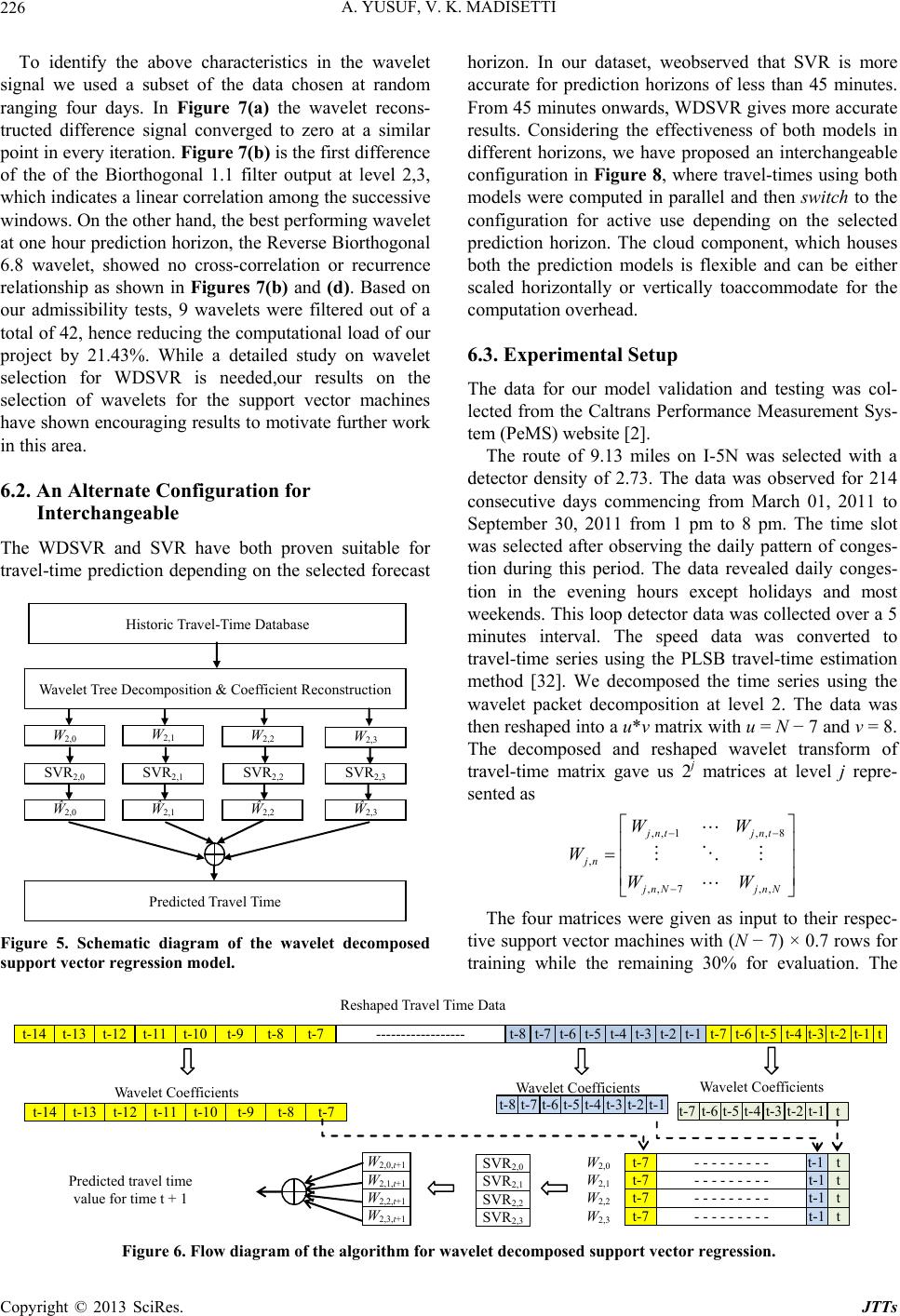

A. YUSUF, V. K. MADISETTI

226

s subset of the data chosen at random

ranging four days. In Figure 7(a) the wavelet recons-

tructed difference signal converged to zero at a similar

p the first difference

wong the successive

windows. On the other hand, the best performing wavelet

at one hour prediction horizon, the Reverse Biorthogonal

rp as shown in Figures 7(b) and (d). Based on

our admout of a

total ofd our

pn wavelet

selection for WDSVR is needed,our results on the

haver work

To identify the above characteristics in the wavelet

ignal we used a

oint in every iteration. Figure 7(b) is

f the of the Biorthogonal 1.1 filter output at level 2,3,

hich indicates a linear correlation am

.8 wavelet, showed no cross-correlation or recurrence

elationshi

issibility tests, 9 wavelets were filtered

42, hence reducing the computational loa of

roject by 21.43%. While a detailed study o

election of wavelets for the support vector machines

shown encouraging results to motivate furthe

n this area.

6.2. An Alternate Configuration for

Interchangeable

The WDSVR and SVR have both proven suitable for

travel-time prediction depending on the selected forecast

Historic Travel-Time Database

Wavelet Tree Decomposition & Coefficient Reconstruction

2,2

2,1

2,0

2,3

SVR

2,2

SVR

2,1

SVR

2,0

SVR

2,3

2,2

2,1

2,0

2,3

Predicted Travel Time

Figuram of the wavelet decomposed

horizon. In our dataset, weobserved that SVR is more

accurate for prediction horizons of less than 45 minutes.

From 45 minutes onwards, WDSVR gives more accurate

results. Considering the effectiveness of both models in

different horizons, we have proposed an interchangeable

configuration in Figure 8, where travel-times using both

models were computed in parallel and then switch to the

configuration for active use depending on the selected

prediction horizon. The cloud component, which houses

both the prediction models is flexible and can be either

scaled horizontally or vertically toaccommodate for the

computation overhead.

6.3. Experimental Setup

ance Measurement Sys-

tem (PeMS) website [2].

The route of 9.13 miles on I-5N was selected with a

detector density of 2.73. The data was observed for 214

consecutive days commencing from March 01, 2011 to

September 30, 2011 from 1 pm to 8 pm. The time slot

was selected after observing the daily pattern of conges-

tion during this period. The data revealed daily conges-

tion in the evening hours except holidays and most

weekends. This loop detector data was collected over a 5

minutes interval. The speed data was converted to

travel-time series using the PLSB travel-time estimation

method [32]. We decomposed the time series using the

wavelet packet decomposition at level 2. The data was

then reshaped into a u*v matrix with u = N − 7 and v = 8.

The decomposed and reshaped wavelet transform of

travel-time matrix gave us 2j matrices at level j repre-

sented as

The data for our model validation and testing was col-

lected from the Caltrans Perform

,, 1,,8

,,7,,

































jnt jnt

jnN jnN

The four matrices were given as input to their respec-

tive support vector machines with (N − 7) × 0.7 rows for

training while the remaining 30% for evaluation. The

re 5. Schematic diag

support vector regression model.

t-8 t-7t-6 t-5 t-4t-3 t-2 t-1

t-14 t-13 t-12 t-11 t-10 t-9 t-8 t-7

SVR

2,0

SVR

2,1

SVR

2,2

SVR

2,3

2,0,t+1

2,1,t+1

2,2,t+1

2,3,t+1

Predicted travel time

value for time t + 1

2,0

t-7- - - - - - - - - t-1 t

2,1

t-7- - - - - - - - - t-1t

2,2

t-7- - - - - - - - - t-1t

2,3

t-7- - - - - - - - - t-1t

t-7 t-6 t-5 t-4 t-3 t-2 t-1 t

t-14 t-13 t-12 t-11 t-10 t-9 t-8 t-7 ------------------ t-8 t-7 t-6 t-5 t-4 t-3t-2 t-1 t-7 t-6 t-5 t-4 t-3 t-2t-1t

Reshaped Travel Time Data

Wavelet Coefficients Wavelet Coefficients Wavelet Coefficients

Figure 6. Flow diagram of the algorithm for wavelet deco mpose d suppor t vector regression.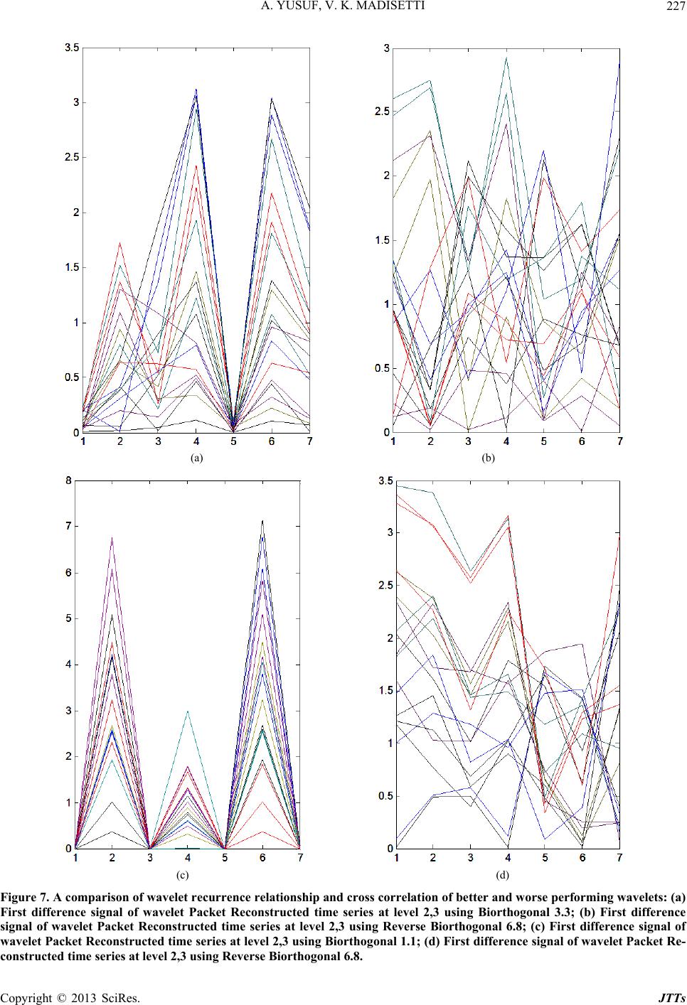

A. YUSUF, V. K. MADISETTI 227

(a) (b)

Figure 7. A comparison of wavelet recurrence relationship and cross correlation of better and worse performing wavelets: (a)

First difference signal of wavelet Packet Reconstructed time series at level 2,3 using Biorthogonal 3.3; (b) First difference

signal of wavelet Packet Reconstructed time series at level 2,3 using Reverse Biorthogonal 6.8; (c) First difference signal of

wavelet Packet Reconstructed time series at level 2,3 using Biorthogonal 1.1; (d) First difference signal of wavelet Packet Re-

constructed time series at level 2,3 using Reverse Biorthogonal 6.8.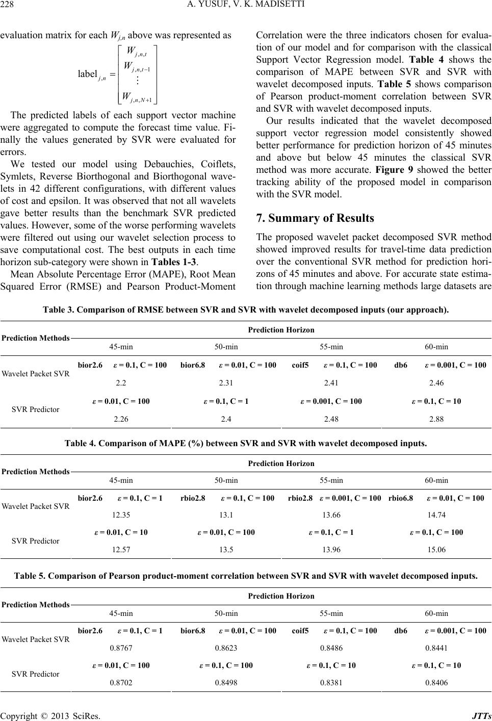

A. YUSUF, V. K. MADISETTI

228

evaluation matrix for each Wj,n above was represented as

The predicted labels of each support vector machine

were aggregated to compute the forecast time value. Fi-

nally the values generated by SVR were evaluated for

errors.

We tested our model using Debauchies, Coiflets,

Symlets, Reverse Biorthogonal and Biorthogonal wave-

lets in 42 different configurations, with different values

of cost and epsilon. It was observed that not all wavelets

gave better results than the benchmark SVR predicted

values. However, some of the worse performing wavelets

were filtered out using our wavelet selection process to

save computational cost. The best outputs in each time

horizon sub-category were shown in Tables 1-3.

Mean Absolute Percentage Error (MAPE), Root Mean

Squared Error (RMSE) and Pearson Product-Moment

Correlation were the three indicators chosen for evalua-

tion of our model and for comparison with the classical

Support Vector Regression model. Table 4 shows the

comparison of MAPE between SVR and SVR with

wavelet decomposed inputs. Table 5 shows comparison

of Pearson product-moment correlation between SVR

and SVR with wavelet decomposed inputs.

Our results indicated that the wavelet decomposed

support vector regression model consistently showed

better performance for prediction horizon of 45 minutes

and above but below 45 minutes the classical SVR

method was more accurate. Figure 9 showed the better

tracking ability of the proposed model in comparison

with the SVR model.

7. Summary of Results

The proposed wavelet packet decomposed SVR method

showed improved results for travel-time data prediction

over the conventional SVR method for prediction hori-

zons of 45 minutes and above. For accurate state estima-

tion through machine learning methods large datasets are

Table 3. Comparison of RMSE betwee n SVR and SVR with wavele t de c o mpose d inputs (our appr oac h).

tion Horizon

,,1

,, 1

label 















jnt

jnN

Predic

Prediction Methods

45-min 60-min 50-min 55-min

bior2.6 ε = 0.1, C = 100 bior6.8 ε = 0.01, C = 100coif5 ε = 0.1, C = 100 db6 ε = 0.001, C = 100

Wavelet Packet SVR

2.2 2.31 2.41 2.46

ε = 0.01, C = 100 ε = 0.1, C = 1 ε = 0.001, C = 100 ε = 0.1, C = 10

SVR Predictor

2.26 2.4 2.48 2.88

Table 4. Comparison of MAPE (%) between SVR and SVR with wavele t decomposed inputs.

Prediction Horizon

Prediction Methods

45-min 50-min 55-min 60-min

bior2.6 ε = 0.1, C = 1 rbio2.8 ε = 0.1, C = 100rbio2.8ε = 0.001, C = 100 rbio6.8 ε = 0.01, C = 100

Wavelet Packet SVR

12.35 13.1 13.66 14.74

ε = 0.01, C = 10 ε = 0.01, C = 100 ε = 0.1, C = 1 ε = 0.1, C = 100

SVR Predictor

12.57 13.5 13.96 15.06

Table 5. Comparison of Pearson product-moment correlation between SVR and SVR with wavelet decomposed inputs.

Prediction Horizon

Prediction Methods

45-min 50-min 55-min 60-min

bior2.6 ε = 0.1, C = 1 bior6.8 0coif5 ε = 0.1, C = 100 db6 ε = 0.001, C = 100ε = 0.01, C = 10

Wavelet Packet SVR

0.870.8441 67 0.8623 0.8486

ε = 0.01, C = 100 ε = 0.1, C = 100 ε = 0.1, C = 10 ε = 0.1, C = 10

SVR Predictor

0.8702 0.8498 0.8381 0.8406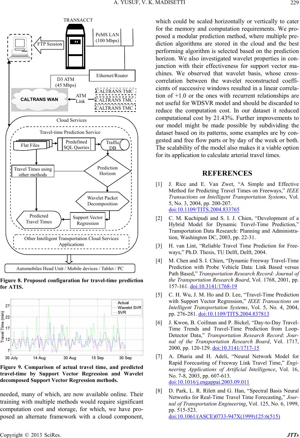

A. YUSUF, V. K. MADISETTI 229

PeMS LAN

(100 Mbps)

D3 ATM

(45 Mbps)

AT M

Link

FTP Session

CALTRANS TMC

TRANSACCT

Ethernet/Router

Cloud Services

Travel-time Prediction Service

Automobiles Head Unit / devices / Tablet / PC Mobile

Flat Files Traffic

Predefined

SQL Queries

Wavelet Packet

Decomposition

Support Vector

ession Regr

Predicte

Travel Tim

Travel Times using

other methods

Other Intelner

Applications

ligent Trasportation Cloud Svices

Prediction

Horizon

CALTRANS WAN

Figure 8. Propo

for ATIS.

sed configuration for travel-time prediction

Fig

travel-time by Support Vector Regression and Wavelet

rt Vector Regression methods.

needed, many of wle T

iple methods would require significant

computation cost and stowhich, we have

posed an alternate framework with a cloud component,

r the memory and computation requirements. We pro-

ucted coeffi-

tterns, some examples are by con-

by day of the week or both.

so makes it a viable option

, Vol.

/TITS.2004.833765

ure 9. Comparison of actual travel time, and predicted

decomposed Suppo

hich, are now availab online.heir

training with mult

rage, for pro-

which could be scaled horizontally or vertically to cater

posed a modular prediction method, where multiple pre-

diction algorithms are stored in the cloud and the best

performing algorithm is selected based on the prediction

horizon. We also investigated wavelet properties in con-

junction with their effectiveness for support vector ma-

chines. We observed that wavelet basis, whose cross-

correlation between the wavelet reconstr

ents of successive windows resulted in a linear correla-

tion of +1.0 or the ones with recurrent relationships are

not useful for WDSVR model and should be discarded to

reduce the computation cost. In our dataset it reduced

computational cost by 21.43%. Further improvements to

our model might be made possible by subdividing the

dataset based on its pa

gested and free flow parts or

The scalability of the model al

for its application to calculate arterial travel times.

REFERENCES

[1] J. Rice and E. Van Zwet, “A Simple and Effective

Method for Predicting Travel Times on Freeways,” IEEE

Transactions on Intelligent Transportation Systems

5, No. 3, 2004, pp. 200-207.

doi:10.1109

i and S. I. J. Chien, “Development of a

Hybrid M Dynamic Travel-rediction,”

Transportation ch: Planning and

ionhin1.

[3] H. van Lint,liable Travel Time Pren for Free-

ways,” Ph.D. Thesis, TU Delft, Delft, 2004.

[4] M. Ch, “Dynamicl-Time

Prediction wcle Data: Lased versus

Path Based,” Transportation Research Record: Journal of

1768, 2001, pp.

[2] C. M. Kuchipud

odel forTime P

Data Resear

gton DC, 2003, pp

Administra-

t, Was. 22-3

“Redictio

en and S. I. Chien Freeway Trave

ith Probe Vehiink B

the Transportation Research Board, Vol.

157-161. doi:10.3141/1768-19

[5] C. H. Wu, J. M. Ho and D. Lee, “Travel-Time Prediction

with Support Vector Regression,” IEEE Transactions on

Intelligent Transportation Systems, Vol. 5, No. 4, 2004,

pp 3. 276-281. doi:10.1109/TITS.2004.8 7813

[6] J. Kwon, B.an and P. Bickel, “Day Travel-

Time Tren Travel-Time Predicom Loop-

Detecto sportation Re Jour-

nal of the Transportation Research Board, Vol. 1717,

2000, pp. 1. doi:10.3141/1717-15

Coifm

ds and

y-to-Da

tion fr

r Data,” Transearch Record:

20-129

[7] A. Dharia and H. Adeli, “Neural Network Model for

neering Applications of Artificial Intelligence, Vol. 16,

03, pp. 607-613.

doi:10.1016 .011

Rapid Forecasting of Freeway Link Travel Time,” Eng

No. 7-8, 20

/j.engappai.2003.09

[8] D. Park, L. Han, “Spectral Basis Neural

e fovee F-

nal of Transportation Engineering, Volo. 6, 1999,

pp. 515-52

doi:10.1061/(ASCE)0733-947X(1999)125:6(515)

R. Rilett and G.

Ntworksr Real-Time Tral Timorecasting,” Jour

. 125, N

A. YUSUF, V. K. MADISETTI

230

[9] D. J. Park and L. sting Multi

nk Trav

works,” In: Land Use and Transportation Plannin

Programming Applications, 1998, pp. 163-170.

[10] L. R. Rilett and D. Park, “Direct Forecasting of Freeway

Corridor Travel Times Using Spectral Basis Neural Net-

works,” Transportation Research Record: Journal of the

Transportation Research Board, Vol. 1752, 2001, pp.

140-147.

[11] C. Cortes and V. Vapnik, “Support-Vector Networks,”

Machine Learning, Vol. 20, No. 3, 1995, pp. 273-297.

doi:10.1007/BF00994018

R. Rilett, “Foreca

el Times Using Modular Neural Net-

ple-Period

Freeway Li

g and

[12] V. N. Vapnik, “The Nature of Statistical Learning The-

ory,” Springer Verlag, Berlin, 2000.

doi:10.1007/978-1-4757-3264-1

[13] V. Vapnik, S. E. Golowich and A. Smola, “Support Vec-

tor Method for Function Approximation, Regression Es-

timation, and Signal Processing,” Advances in Neural In-

formation Processing Systems, Vol. 9, 1997, pp. 281-287.

[14] T. B. Trafalis and H. Ince, “Support Vector Machine for

Regression and Applications to Financial Forecasting,”

IJCNN 2000, Proceedings of the IEEE International Joint

Conference on Neural Networks, Como, 27 July 2000, pp.

348-353.

[15] M. Song, C. M. Breneman, J. Bi, N. Sukumar, K. P.

Bennett, S. Cramer and N. Tugcu, “Prediction of Protein

Retention Times in Anion-Exchange Chromatography

Systems Using Support Vector Regression,” Journal of

Chemical Information and Computer Sciences, Vol. 42,

No. 6, 2002, pp. 1347-1357. doi:10.1021/ci025580t

[16] F. Wang, G. Tan and Y. Fang, “Multiscale Wavele

port Vector Regression for Traffic Flow Prediction,” 3rd

International Symposium on Intelligent Information Te-

chnology Application (IITA 2009), Nanchang, 21-22 No-

vember 2009, pp. 319-322.

[17] S. Yao, C. Hu and W. Peng, “Server Load Prediction

Based on Wavelet Packet and Support Vector Regression,”

2006 International Conference on Computational Intelli-

gence and Security, Guangzhou, 3-6 November 2006, pp

1016-1019.

ssion based S-Transform,” IASTED, International

Conference on Modelling, Simulation, and Identifica-

tion/658: Power and Energy Systems/660, 661, 662, Bei-

jing, 2009.

[19] H. van Lint, S. P. Hoogendoorn and H. J. van Zu

“State Space Neural Networks for Freeway Travel Time

Prediction,” In: J. R. Dorronsoro, Ed., Artificial Neural

Networks—ICANN 2002, Madrid, 28-30 August 2002, pp

1043-1048.

[20] S. Innamaa, “Short-Term Prediction of Travel Time Us-

ing Neural Networks on an Interurban Highway,” Trans-

t Sup-

[18] M. Faisal and A. Mohamed, “A New Technique to Pre-

dict the Sources of Voltage Sags using Support Vector

Regre

ylen,

portation, Vol. 32, No. 6, 2005, pp. 649-669.

doi:10.1007/s11116-005-0219-y

[21] J. W. C. van Lint, “Reliable Real-Time Framework for

Short-Term Freeway Travel Time Prediction,” Journal of

921-93

doi:10.1061

Transportation Engineering, Vol. 132, No. 12, 2006, pp.

/(ASCE)0733-947X(2006)132:12(921)

[22] N. Zou, J. Wg and G. L. Chang, “A Reliable Hybrid . Wan

Prediction Model for Real-Time Travel Time Prediction

with Widely Spaced Detectors,” 11th International IEEE

Conference on Intelligent Transportation Systems, Bei-

jing, 12-15 October 2008, pp. 91-96.

[23] N. Zou, J. W. Wang, G. L. Chang and J. Paracha, “Ap-

plication of Advanced Traffic Information Systems Field

Test of a Travel-Time Prediction System with Widely

Spaced Detectors,” Transportation Research Record: Jour-

nal of the Transportation Research Board, Vol. 2129,

2009, pp. 62-72. doi:10.3141/2129-08

[24] J. W. C. van Lint, S. P. Hoogendoorn and H. J. van

Zuylen, “Accurate Freeway Travel Time Prediction with

State-Space Neural Networks under Missing Data,” Tran-

sportation Research Part C: Emerging Technologies, Vol.

13, No. 5-6, 2005, pp. 347-369.

doi:10.1016/j.trc.2005.03.001

[25] H. J. M. Van Grol, M. Danech-Pajouh, S. Manfredi and J.

Whittaker, “DACCORD: On-Line Travel Time Predic-

tion,” World Transport Research: Selected Proceedings

of the 8th World Conference on Transport Research,

Pergamon, Oxford, 1999.

[26] H. Chen, M. S. Dougherty and H. R. Kirby, “The Effects

of Detector Spacing on Traffic Forecasting Performance

Using Neural Networks,” Computer-Aided Civil and In-

frastructure Engineering, Vol. 16, No. 6, 2001, pp. 422-

430. doi:10.1111/0885-9507.00244

[27] P. Yi, S. Dinglor, “Investigating

tor Spacing and Sample

, H. Wei and G. W. Say

the Effect of Detector Spacing on Midpoint-Based Travel

Time Estimation,” Journal of Intelligent Transportation

Systems, Vol. 13, No. 3, 2009, pp. 149-159.

[28] J. Kwon, K. Petty and P. Varaiya, “Probe Vehicle Runs or

Loop Detectors?: Effect of Detec

Size on Accuracy of Freeway Congestion Monitoring,”

Transportation Research Record: Journal of the Trans-

portation Research Board, Vol. 2012, 2007, pp. 57-63.

doi:10.3141/2012-07

[29] C. Chen, J. Kwon, J. Rice, A. Skabardonis and P. Varaiya,

“Detecting Errors and Imputing Missing Data for Single-

Loop Surveillance Systems,” Transportation Research

Record: Journal of the Transportation Research Board,

Vol. 1855, 2003, pp. 160-167. doi:10.3141/1855-20

[30] L. N. Jacobson, N. L. Nihan and J. D. Bender, “Detecting

Erroneous Loop Detector Data in a Freeway Traffic Man-

agement System,” Transportation Research Record, Wa-

cord: Jour-

shington DC, 1990.

[31] C. D. R. Lindveld, R. Thijs, P. H. L. Bovy and N. J. Van

der Zijpp, “Evaluation of Online Travel Time Estimators

and Predictors,” Transportation Research Re

nal of the Transportation Research Board, Vol. 1719,

2000, pp. 45-53. doi:10.3141/1719-06

[32] J. W. C. van Lint and N. Van der Zijpp, “Improving a

Travel-Time Estimation Algorithm by Using Dual Loop

Detectors,” Transportation Research Record: Journal of

the Transportation Research Board, Vol. 1855, 2003, pp.

41-48. doi:10.3141/1855-05

[33] M. Saito and T. Watanabe, “Prediction and Dissemination

A. YUSUF, V. K. MADISETTI

231

ilizing Vehicle Detect

ort Systems World

nsportation Engineering, Vol. 129, No. 6,

System for Travel Time Ut

Steps Forward: Intelligent Transp

ors,”

Congress, Yokohama, 9-11 November 1995, p. 106.

[34] I. Steven, J. Chien and C. M. Kuchipudi, “Dynamic Travel

Time Prediction with Real-Time and Historic Data,”

Journal of Tra

2003, p. 608.

doi:10.1061/(ASCE)0733-947X(2003)129:6(608)

[35] X. Zhang and J. A. Rice, “Short-Term Travel Time Pre-

diction,” Transportation Research Part C: Emerging

Technologies, Vol. 11, No. 3-4, 2003, pp. 187-210.

doi:10.1016/S0968-090X(03)00026-3

[36] H. Sun, H. X. Liu, H. Xiao, R. R. He and B. Ran, “Use of

Local Linear Regression Model for Short-Term Traffic

Forecasting,” Transportation Research Record: Journal

of the Transportation Research Board, Vol. 1836, 2003,

pp. 143-150. doi:10.3141/1836-18

[37] M. S. Ahmed and A. R. Cook, “Analysis of Freewa

Traffic Time-Series Data

by Using Box-Jenkins Tech-

orecasting Freeway Oc-

niques,” Transportation Research Record, No. 722, 1979,

pp. 1-9.

[38] M. Levin and Y. D. Tsao, “On F

cupancies and Volumes (Abridgment),” Transportation

Research Record, No. 722, 1980, pp. 47-49.

[39] T. Oda, “An Algorithm for Prediction of Travel Time

Using Vehicle Sensor Data,” Third International Confer-

ence on Road Traffic Control, London, 1-3 May 1990, pp.

40-44.

[40] M. P. D’Angelo, H. M. Al-Deek and M. C. Wang,

“Travel-Time Prediction for Freeway Corridors,” Trans-

portation Research Record: Journal of the Transportation

Research Board, Vol. 1676, 1999, pp. 184-191.

doi:10.3141/1676-23

[41] S. Ishak and H. Al-Deek, “Performance Evaluation of

Short-Term Time-Series Traffic Prediction Model,” Jour-

nal of Transportation Engineering, Vol. 128, No. 6, 2002,

pp. 490-498.

doi:10.1061/(ASCE)0733-947X(2002)128:6(490)

[42] H. F. Ji, A. G. Xu, X. Sui and L. Y. Li, “The Applied

Research of Kalman in the Dynamic Travel Time Predic-

tion,” Geoinformatics, 2010 18th Internation

ence on, Beijing, 18-20 June 2010, pp

al Confer-

. 1-5.

rent Neural Networks,” Advanced Traffic

ignal

ravel Time Predic-

[43] J. W. C. van Lint, S. P. Hoogendoorn and H. J. van

Zuylen, “Freeway Travel Time Prediction with State-

Space Neural Networks-Modeling State-Space Dynamics

with Recur

Management Systems for Freeways and Traffic S

Systems 2002: Highway Operations, Capacity, and Traf-

fic Control, No. 1811, 2002, pp. 30-39.

[44] C. P. I. van Hinstiergen, J. W. C. van Lint and H. J. van

Zuylen, “Bayesian Training and Committees of State-

Space Neural Networks for Online T

tion,” Transportation Research Record, Vol. 2105, 2009,

pp. 118-126. doi:10.3141/2105-15

[45] D. Park, L. R. Rilett and G. H. Han, “Forecasting Multi-

ple-Period Freeway Link Travel Times Using Neural

Networks with Expanded Input Nodes,” Applications of

Advanced Technologies in Transportation, No. 1617,

H. Koutsopoulos and R.

i, “Network State Estimation

1998, pp. 325-332.

[46] L. Vanajakshi and L. R. Rilett, “Support Vector Machine

Technique for the Short Term Prediction of Travel Time,”

2007 IEEE Intelligent Vehicles Symposium, Istanbul, 13-

15 June 2007, pp. 600-605.

[47] M. Ben-Akiva, M. Bierlaire,

Mishalani, “DynaMIT: A Simulation-Based System for

Traffic Prediction,” DACCORD Short Term Forecasting

Workshop, Delft, 1998.

[48] M. Ben-Akiva, M. Bierlaire, D. Burton, H. N. Kout-

sopoulos and R. Mishalan

and Prediction for Real-Time Traffic Management,” Net-

works and Spatial Economics, Vol. 1, No. 3-4, 2001, pp.

293-318. doi:10.1023/A:1012883811652

[49] S. G. Mallat, “A Wavelet Tour of Signal Processing,”

Academic Press, Edinburgh, 1999.

[50] M. Vetterli and J. Kovačević, “Wavelets and Subband

Coding,” Prentice Hall-PTR, Upper Saddle River, 1995.
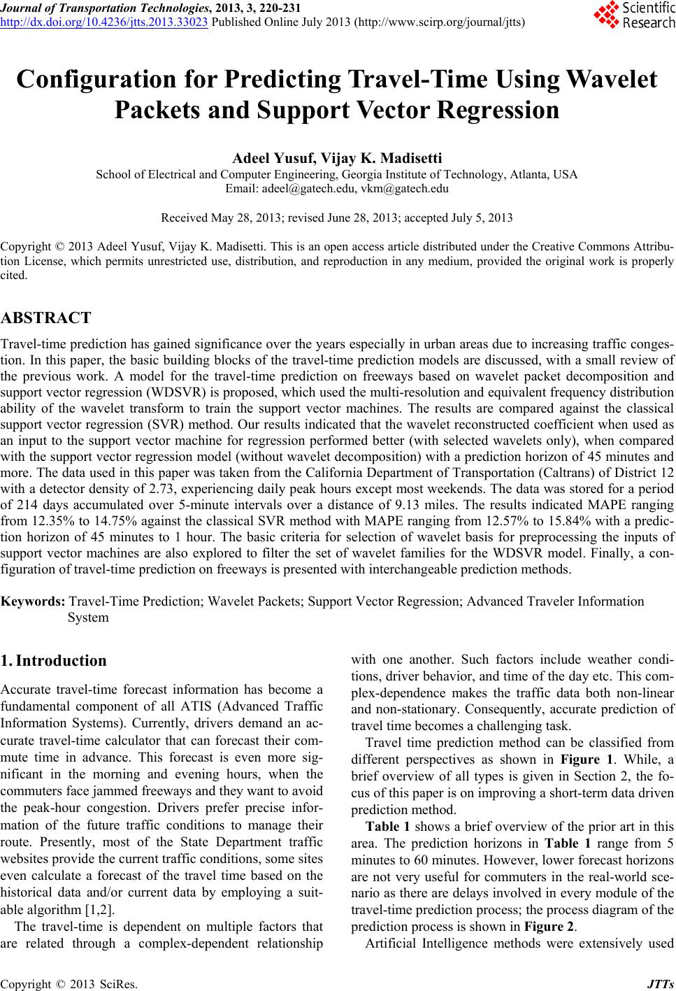