Vol.2, No.12, 1386-1393 (2010)
doi:10.4236/ns.2010.212169
Copyright © 2010 SciRes. Openly accessible at http:// www.scirp.org/journal/NS/
Natural Science
Modeling of unsteady MHD free convection flow with
radiative heat transfer in a rotating fluid
Harouna Naroua
Département de Mathématiques et Informatique, Université Abdou Moumouni, Niamey, Niger;
Received 4 October 2010; revised 5 November 2010; accepted 10 November 2010.
ABSTRACT
In this paper, a numerical simulation has been
carried out on unsteady hydromagnetic free
convection near a moving infinite flat plate in a
rotating medium. The temperatures involved are
assumed to be very high so that the radiative
heat transfer is significant, which renders the
problem highly non-linear even with the as-
sumption of a differential approximation for the
radiative heat flux. A numerical method based
on the Naka mura scheme has been employ e d to
obtain the temperature and velocity distribu-
tions which are depic ted graph ically. The effects
of the different parameters entering into the
problem have been discussed extensively.
Keywords: Modeling; Numerical Simulation;
Nakamura Scheme;
Unsteady Hydrom agn etic Free Con vect i on;
Radiative Heat Transfer; Computer Prog ram
1. INTRODUCTION
In recent years, an extensive research effort has been
directed towards the theory of rotating fluids owing to its
numerous applications in cosmical and geophysical fluid
dynamics, meteorology and engineering [1]. Batchelor
[2] studied the Ekman layer flow on a horizontal plate.
The flow past a horizontal plate has also been studied by
Debnath [3-5], Puri and Kulshrestha [6], Tokis and Ge-
royannis [7]. Investigations on the flow past a vertical
plate have been carried out by Tokis [8], Kythe and Puri
[9]. Though various methods exist for solving fluid flow
problems, Naroua et al. [10-11] presented a finite ele-
ment approach. The problem of thermal radiation has
been approached by Ghosh and Pop [12], Raptis and
Perdikis [13].
Since high temperature phenomenon abound in solar
physics, particularly in astrophysical studies, radiation
effects cannot be neglected. This paper therefore incor-
porates radiative transfer into the studies, thereby wid-
ening the applicability of the results. For an optically
thin gas, which is approximated by a transparent me-
dium, the absorption coefficient (which will be assumed
constant in the analysis) α >> 1 and the radiative flux Q'
satisfies the non-linear differential equation (Cheng [14])

44
4
QTT
z





 

(1)
where T' is the temperature of the fluid, subscript ∞ will
be used to denote conditions in the undisturbed fluid and
σ is the Stefan-Boltzmann constant.
2. MATHEMATICAL ANALYSIS
Consider the unsteady flow of an electrically-conducting
incompressible viscous fluid past a vertical flat plate
which moves in its own plane with velocity U0 and ro-
tates about the z' axis with angular velocity Ω. The plate
is maintained at


1TT


ww . Following the arguments
given by Tokis [8] and employing Eq.1, the governing
equations for a transparent medium are as follows:

2
2
0
2
2c
uu
vBugT
tz




T





 


(2)
2
2
0
2
2c
vv
u
tz




B v


 

 (3)

2
44
24
p
TT
Ck TT
tz


  
 
 

0
(4)
where (u', v', 0) are the velocity components, k is the
thermal conductivity, g is the gravitational acceleration,
σc is the electrical conductivity, υ is the kinematic vis-
cosity, β0 is the coefficient of volumetric thermal expan-
sion and Cp is the specific heat at constant pressure.
The boundary conditions are:
0,0,
0, 0,
w
uUvT Tonz
uvTTasz




 
 

 
(5)

H. Naroua / Natural Science 2 (2010) 1386-1393
Copyright © 2010 SciRes. Openly accessible at http://www.scirp.org/journal/NS/
1381387
Introducing the following non-dimensional quantities:




2
00
0
2
20
22
00
3
32
00
, ,
,,, ,,
,Pr,,
4
,
w
w
pc
c
p
TT uv
tU zU
tz uv
U
CB
EM
k UU
T
gT
Gr R
UCU


 






 
,
T

  

 





 
 





(6)
The Eqs.2-5 reduce to:


2
2
2
2
4
2
21(7)
Pr1 (8)
qq
iEqM qGr
tz
R
tz

 

 





 


z
z
where q = u + iv and
1, 0
0, 0
w
qat
qas


 

 
 (9)
Using q = u + iv, the system of Eqs.7,8 becomes:


2
2
2
2
2
2
2
4
2
21 (10)
2 (11)
Pr1 (12)
uu
EvMuGr
tz
vv
EuMv
tz
R
tz

 

 









 


The above system of Eqs.10-12 with boundary condi-
tions (9) has been solved numerically by a computer
program using a finite-difference scheme as described by
Nakamura [15]. The mesh system is shown in Figure 1.
Eqs.10-12 are coupled non-linear parabolic partial
differential equations in u, v and Ө. We first discretise
them using the backward difference approximation
(which is stable) in the time coordinate as shown in Eqs.
13-15:

,1
2
,1
2
3
,1
112 (13)
12 (14)
Pr Pr (15)
ij
ij
ij
u
uM uGrEv
tt
v
vM vEu
tt
RR
tt

 




  







  






  




where ,,uv



are derivatives with respect to z.
For the sake of simplicity, we write:
2
21 0
1
1; 0;;BBBM
t

 



2
21 0
1
1; 0;;CCCM
t

 



3
21 0
Pr
1; 0;DDDR
t


 



Using the above formulation, Eqs.13-15 take the
form:

2, 1,0,,,1,
2, 1,0,,,1
2, 1, 0,,1
1
12 (16)
1
2 (17)
Pr (18)
ij ijijijijij
ij ijijijij
ij ijijij
Bu BuBuGruEv
t
Cv Cv CvEuv
t
DDD R
t

 



 
 




 
 



 
 





Using the central difference scheme which is uncondi
tio
-
nally stable, Eqs.16-18 reduce to:



1,, 1,1, 1,
210,,,1,
2
1,,1,1, 1,
210,,,1
2
1, ,
2
21
12
2
21
2
2
2
ijij ijij ij
ijij ijij
ijij ijij ij
ijij ij
ijij i
uuu uu
BBBuGruEv
zt
z
vvv vv
CCCvEuv
zt
z
D








 









 










(19)
(20)
1,1, 1,
10,,1
2
Pr (21)
2
jijij
ij ij
DD R
zt
z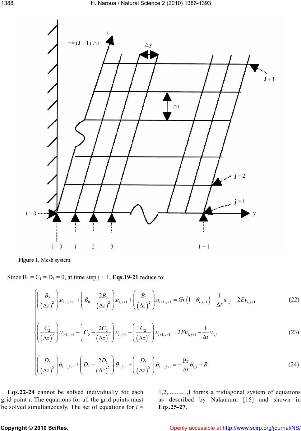
 

























H. Naroua / Natural Science 2 (2010) 1386-1393 1388
Figure 1. Mesh system.
Since B1 = C1 = D1 = 0, at time step j + 1, Eqs.19-21 reduce to:
 

 
222
1, 10, 11, 1,1,, 1
222
222
1, 10, 11,1, 1,
222
2


21
... 12(22)
21
...2 (23)
i jiji jijijij
i jijijijij
BBB
uB uuGruEv
t
zzz
CCC
vCvvEu v
t
zzz
D

 
 
 
   
 

 
 
  
 

 
Copyright © 2010 SciRes. Openly accessible at http:// www.scirp.org/journal/NS/
 
22
0, 11, 1,
22
2Pr
.. (24)
iji jij
DD
DR
t
zz

 











 

 


 

Eqs.22-24 cannot be solved individually for each
grid point i. The equations for all the grid points must
be solved simultaneously. The set of equations for i =
1,2,...........,I forms a tridiagonal system of equations
as described by Nakamura [15] and shown in
Eqs.25-27.
1, 1
2
i j
z





H. Naroua / Natural Science 2 (2010) 1386-1393
Copyright © 2010 SciRes. Openly accessible at http://www.scirp.org/journal/NS/
1381389
 
  
  
 
22
022
222
0
222
222
01
222
22
0
22
2
2
2.
2
BB
B
zz
BBB
B
zzz
BBB
Bs
zzz
BB
B
zz


 






  
 
 
 

 

  
  

 


 



 

  

 

 
f

1 (25)
where and




1, 1
2,1
j
j
u
u






3, 1
1
,1
,1
j
ij
Ij
u
s
u
u

















1, 11,1, 1
2, 12,2, 1
13, 13,3, 1
,1, ,1
1
12
1
12
1
12
1
12
jj
jj
jj
IjIj Ij
Gru Ev
t
Gru Ev
t
fGru Ev
t
Gru Ev
t









 




 










 





j
j
j

 
 
 
 
22
0
222
0
222
222
02
222
22
0
22
2
2
2.
2
CC
C
zz
CCC
C
zzz
CCC
Csf
zzz
CC
C
zz










  
 
 
 

 

  
  

 


 



 

  

 

 





2 (26)
where
v
22


1, 1
2,1
3,1
2
,1
,1
j
j
j
ij
Ij
v
v
s
v
v
































and
1, 11,
2, 12,
23,13
,1 ,
1
2
1
2
1
2
1
2
jj
,
j
j
j
j
I
jI
Eu v
t
Eu v
t
fEu v
t
Eu v
t



























j
 
 
 
 
22
022
222
0
222
222
0
222
22
0
22
2
2
2.
2
DD
D
zz
DDD
D
zzz
DDD
Ds
zzz
DD
D
zz


 






  
 
 
 

 

 

 


 


 



 

  

 

 





33
f

(27)
where
1, 1
2,1
j
j




3,1
3
,1
,1
j
ij
Ij
s

































and
1,
2,
3,
3
,
,
Pr
Pr
Pr
Pr
Pr
j
j
j
ij
Ij
R
t
R
t
R
t
f
R
t
R
t






























 






For each time step, the system of Eqs.25-27 requires
an iterative procedure due to the presence of non-linear
ents. Succetion and iteratio are
continuously executed for each time step until conver-
gence is reached.
3. DISCUSSION OF RESULTS
To get a physical insight into the problem and for the
coefficissive substitun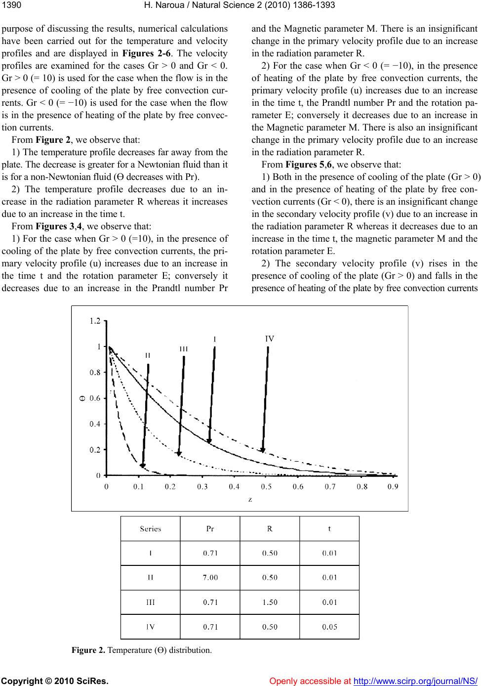

H. Naroua / Natural Science 2 (2010) 1386-1393
Copyright © 2010 SciRes. http://www.scirp.org/journal/NS/
1390
purpose of discussing the results, numerical calculations
have been carried out for the temperature and velocity
profiles and are displayed in Figures 2-6. The velocity
profiles are examined for the cases Gr > 0 and Gr < 0.
Gr > 0 (= 10) is used for the case when the flow is in the
presence of cooling of the plate by free convection cur-
rents. Gr < 0 (= −10) is used for the case when the flow
is in the presence of heating of the plate by free c
tion currents.
From Figure 2, we observe that:
1) The temperature profile decreases far away from the
plate. The decrease is greater for a Newtonian fluid than it
is for a non-Newtonian fluid (Ө decreases with Pr).
2) The temperature profile decreases due to an in-
crease in the radiation parameter R whereas it increases
due to an increase in the time t.
From Figures 3,4, we observe that:
1) For the case when Gr > 0 (=10), in the presence of
cooling of the plate by free convection currents, the pri-
mary velocity profile (u) increases due to an increase in
the time t and the rotation parameter E; conversely it
decreases due to an increase in the Prandtl number Pr
ease
in
onvection currents, the
pr to an increase
in
From Figures 5,6, we observe that:
1) Both in the presence of cooling of the plate (Gr > 0)
and in the presence of heating of the plate by free con-
vection currents (Gr < 0), there is an insignificant change
in the secondary velocity profile (v) due to an increase in
the radiation parameter R whereas it decreases due to an
increase in the time t, the magnetic parameter M and the
rotation parameter E.
2) The secondary velocity profile (v) rises in the
presence of cooling of the plate (Gr > 0) and falls in the
presence of heating of the plate by free convection currents
and the Magnetic parameter M. There is an insignificant
change in the primary velocity profile due to an incr
the radiation parameter R.
2) For the case when Gr < 0 (= −10), in the presence
of heating of the plate by free c
imary velocity profile (u) increases due
the time t, the Prandtl number Pr and the rotation pa-
rameter E; conversely it decreases due to an increase in
the Magnetic parameter M. There is also an insignificant
change in the primary velocity profile due to an increase
in the radiation parameter R.
onvec-
Ө
Figure 2. Temperature (Ө) distribution.
Openly accessible at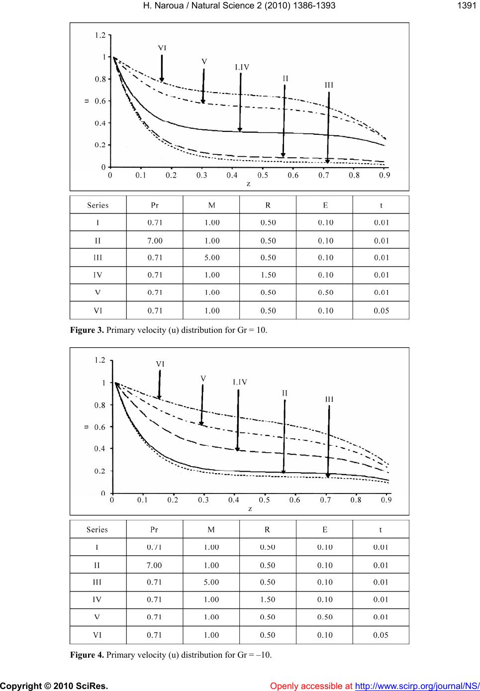

H. Naroua / Natural Science 2 (2010) 1386-1393
Copyright © 2010 SciRes. Openly accessible at http://www.scirp.org/journal/NS/
1391391
Figure 3. Primary velocity (u) distribution for Gr = 10.
Figure 4. Primary velocity (u) distribution for Gr = –10.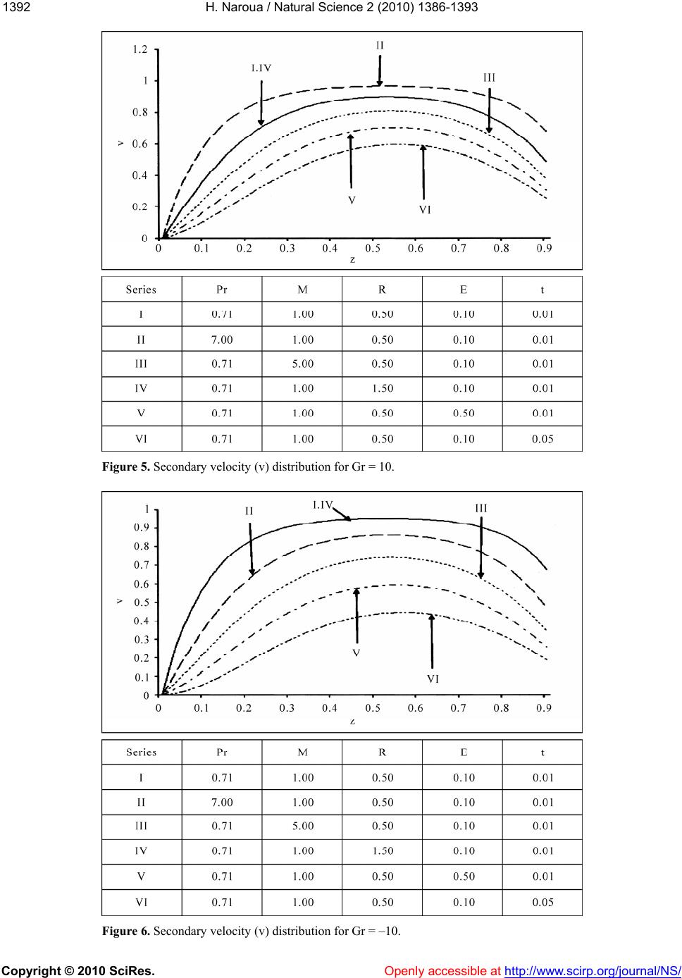

H. Naroua / Natural Science 2 (2010) 1386-1393
Copyright © 2010 SciRes. Openly accessible at http:// www.scirp.org/journal/NS/
1392
Figure 5. Secondary velocity (v) distribution for Gr = 10.
Figure 6. Secondary velocity (v) distribution for Gr = –10.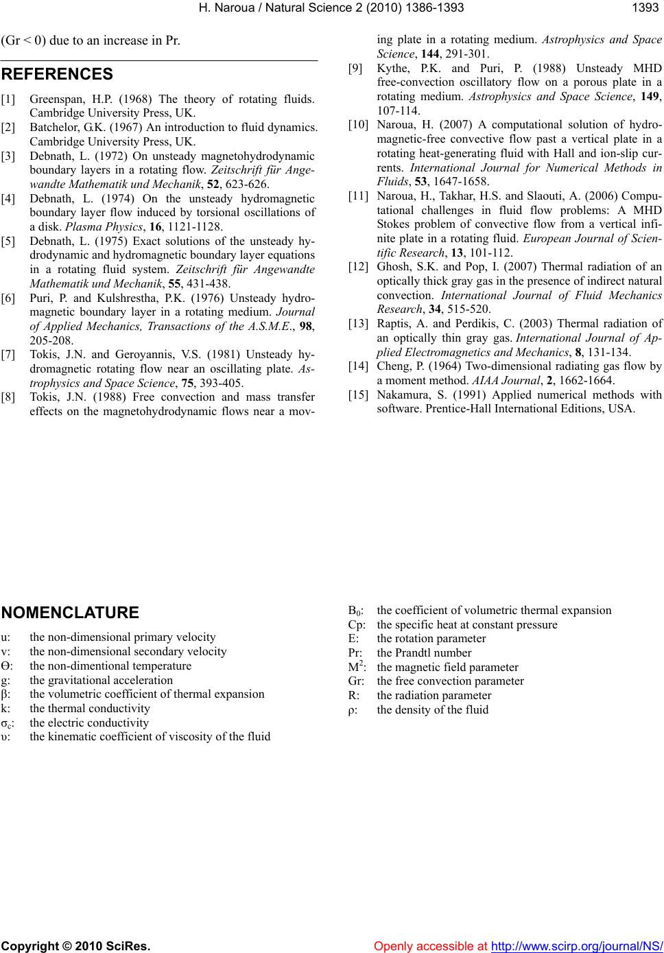

H. Naroua / Natural Science 2 (2010) 1386-1393
Copyright © 2010 SciRes. http:// www.scirp.org/journal/NS/
1391393
(Gr < 0) due to an increase in Pr.
REFERENCES
[1] Greenspan, H.P. (1968) The theory of rotating fluids.
Cambridge University Press, UK.
[2] Batchelor, G.K. (1967) An introduction to fluid dynamics.
Cambridge University Press, UK.
[3] Debnath, L. (1972) On unsteady magnetohydrodynamic
boundary layers in a rotating flow. Zeitschrift für Ange-
wandte Mathematik und Mechanik, 52, 623-626.
[4] Debnath, L. (1974) On the unsteady hydromagnetic
boundary layer flow induced by torsional oscillations of
a disk. Plasma Physics, 16, 1121-1128.
[5] Debnath, L. (1975) Exact solutions of the unsteady hy-
drodynamic and hydromagnetic boundary layer equations
in a rotating fluid system. Zeitschrift für Angewandte
Mathematik und Mechanik, 55, 431-438.
[6] Puri, P. and Kulshrestha, P.K. (1976) Unsteady hydro-
magnetic boundary layer in a rotating medium. Journal
of Applied Mechanics, Transactions of the A.S.M.E., 98,
205-208.
[7] Tokis, J.N. and Geroyannis, V.S. (1981) Unsteady hy-
dromagnetic rotating flow near an oscillating plate. As-
trophysics and Space Science, 75, 393-405.
[8] Tokis, J.N. (1988) Free convection and mass transfer
effects on the magnetohydrodynamic flows near a mov-
ing plate in a rotating medium. Astrophysics and Space
Science, 144, 291-301.
[9] Kythe, P.K. and Puri, P. (1988) Unsteady MHD
tory flow on a porous plate in a
rotating medium. Astrophysics and Space Science, 149,
107-114.
[10] Naroua, H. (2007) A computational solution of hydro-
magnetic-free convective flow past a vertical plate in a
rotating heat-generating fluid with Hall and ion-slip cur-
rents. International Journal for Numerical Methods in
Fluids, 53, 1647-1658.
[11] Naroua, H., Takhar, H.S. and Slaouti, A. (2006) Compu-
tational challenges in fluid flow problems: A MHD
Stokes problem of convective flow from a vertical infi-
nite plate in a rotating fluid. European Journal of Scien-
tific Research, 13, 101-112.
[12] Ghosh, S.K. and Pop, I. (2007) Thermal radiation of an
optically thick gray gas in the presence of indirect natural
convection. International Journal of Fluid Mechanics
Research, 34, 515-520.
[13] Raptis, A. and Perdikis, C. (2003) Thermal radiation of
an optically thin gray gas. International Journal of Ap-
plied Electromagnetics and Mechanics, 8, 131-134.
[14] Cheng, P. (1964) Two-dimensional radiating gas flow by
a moment method. AIAA Journal, 2, 1662-1664.
[15] Nakamura, S. (1991) Applied numerical methods with
software. Prentice-Hall International Editions, USA.
NOMENCLATURE
u: the non-dimensional primary velocity
v: the non-dimensional secondary velocity
Ө: the non-dimentional temperature
g: the gravitational acceleration
β: the volumetric coefficient of thermal expansion
k: the thermal conductivity
σc: the electric conductivity
υ: the kinematic coefficient of viscosity of the fluid
B0: the coefficient of volumetric thermal expansion
Cp: the specific heat at constant pressure
E: the rotation parameter
Pr: the Prandtl number
M2: the magnetic field parameter
Gr: the free convection parameter
R: the radiation parameter
ρ: the density of the fluid
free-convection oscilla
Openly accessible at