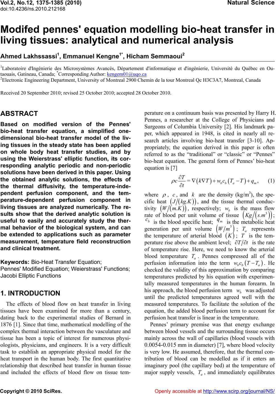
 Vol.2, No.12, 1375-1385 (2010) doi:10.4236/ns.2010.212168 Copyright © 2010 SciRes. Openly accessible at http:// www. scirp.org/journal/NS/ Natural Science Modifed pennes' equation modelling bio-heat transfer in living tissues: analytical and numerical analysis Ahmed Lakhssassi1, Emmanuel Kengne1*, Hicham Semmaoui2 1Laboratoire d'Ingénierie des Microsystèmes Avancés, Département d'informatique et d'ingénierie, Université du Québec en Ou- taouais, Gatineau, Canada; *Corresponding Autho r: kengem01@uqo.ca 2Electronic Engineering Department, University of Montreal 2900 Chemin de la tour Montreal Qc H3C3A7, Montreal, Canada Received 20 September 2010; revised 25 October 2010; accepted 28 October 2010. ABSTRACT Based on modified version of the Pennes' bio-heat transfer equation, a simplified one- dimensional bio-heat transfer model of the liv- ing tissues in the steady state has been applied on whole body heat transfer studies, and by using the Weierstrass' elliptic function, its cor- responding analytic periodic and non-periodic solutions have been derived in this paper. Using the obtained analytic solutions, the effects of the thermal diffusivity, the temperature-inde- pendent perfusion component, and the tem- perature-dependent perfusion component in living tissues are analyzed numerically. The re- sults show that the derived analytic solution is useful to easily and accurately study the ther- mal behavior of the biological system, and can be extended to applications such as parameter measurement, temperature field reconstruction and clinical treatment. Keywords: Bio-Heat Transfer Equation; Pennes' Modified Equation; Weierstrass' Functions; Jacobi Elliptic Functions 1. INTRODUCTION The effects of blood flow on heat transfer in living tissues have been examined for more than a century, dating back to the experimental studies of Bernard in 1876 [1]. Since that time, mathematical modelling of the complex thermal interaction between the vasculature and tissue has been a topic of interest for numerous physi- ologists, physicians, and engineers. It is a very difficult task to establish an appropriate physical model for the heat transport in the human body. The first quantitative relationship that described heat transfer in human tissue and included the effects of blood flow on tissue tem- perature on a continuum basis was presented by Harry H. Pennes, a researcher at the College of Physicians and Surgeons of Columbia University [2]. His landmark pa- per, which appeared in 1948, is cited in nearly all re- search articles involving bio-heat transfer [3-10]. Ap- propriately, the equation derived in this paper is often referred to as the “traditional” or “classic” or “Pennes” bio-heat equation. The general form of Pennes’ bio-heat equation is [7] =, bb am T ckTwcTT t q (1) where , , and are the density (kg/m3), the spe- cific heat ck kg.K , and the tissue thermal conduc- tivity .KWm , respectively; b is the mass flow rate of blood per unit volume of tissue w 3 Kg s.m; c is the blood specific heat; q is the metabolic heat generation per unit volume b m ; represents the temperature of arterial blood 3 Wm a T ; is the tem- perature rise above th e ambient lev el; T Tt T w wc is the rate of temperature rise. Here, we need to know the arterial blood temperature a T. Pennes compressed all of the perfusion information into the term bba . He checked the valid ity of this approxi mation by comparing temperatures predicted by his equation with experimen- tally measured temperatures in the human forearm. In his approach, the blood perfusion term b was adjusted until the predicted temperatures agreed well with the measured temperatures. To facilitate the solution of the equation, the added blood perfusion term to account for perfusion heat transfer is linear in the temperature. T Pennes’ primary premise was that energy exchange between blood vessels and the surrounding tissue occurs mainly across the wall of capillaries (blood vessels with 0.0054-0.015 mm in diameter) [7], where blood velocity is very low. He assumed, therefore, that the thermal con- tribution of blood can be modelled as if it enters an imaginary pool (the capillary bed) at the temperature of major supply vessels, , and immediately equilibrates a T 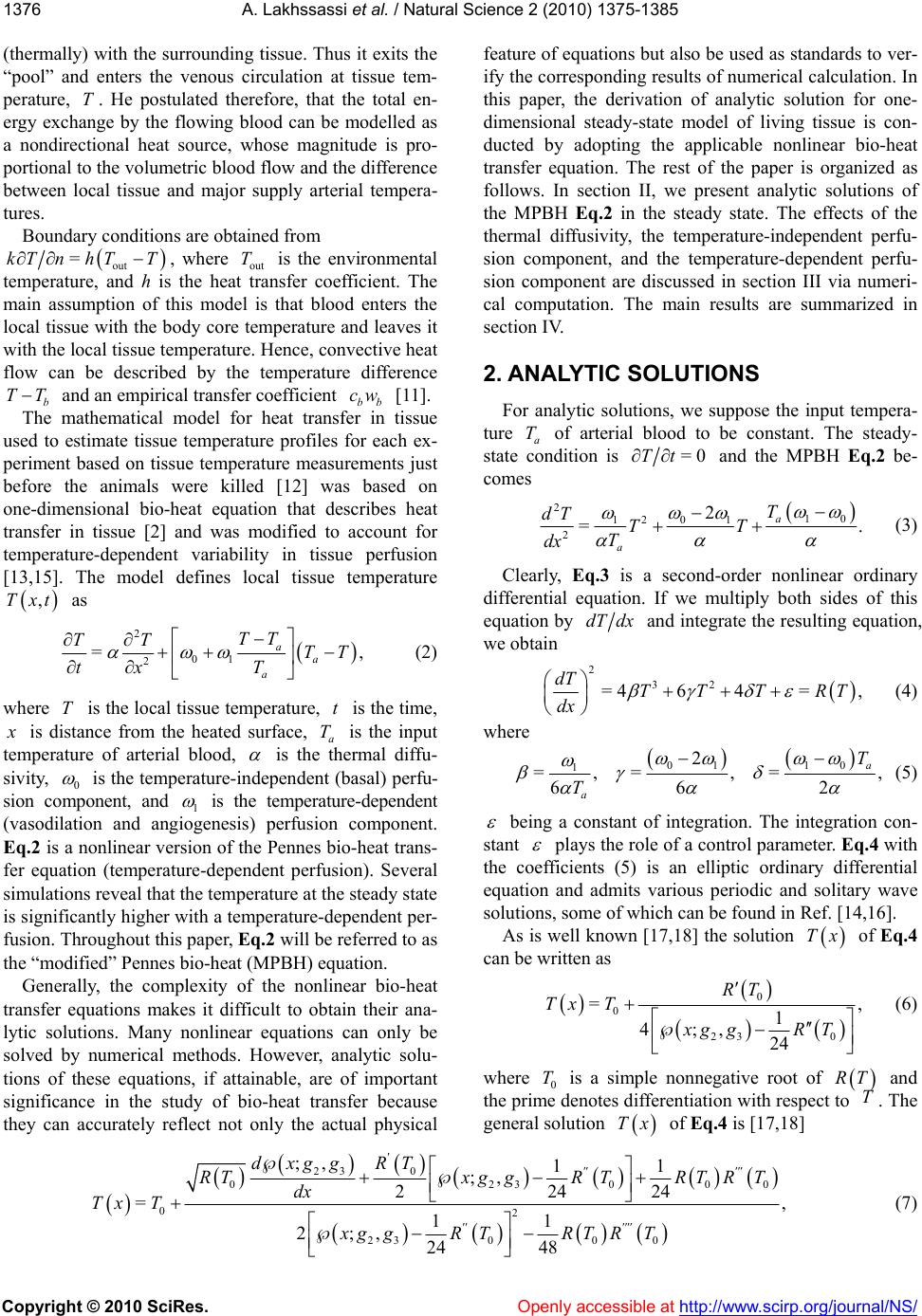 A. Lakhssassi et al. / Natural Science 2 (2010) 1375-1385 Copyright © 2010 SciRes. Openly accessible at http://www.scirp.org/journal/NS/ 1376 (thermally) with the surrounding tissue. Thus it exits the “pool” and enters the venous circulation at tissue tem- perature, . He postulated therefore, that the total en- ergy exchange by the flowing blood can be modelled as a nondirectional heat source, whose magnitude is pro- portional to the volumetric blood flow and the difference between local tissue and major supply arterial tempera- tures. T Boundary conditions are obtained from out kT nTT =h, where out is the environmental temperature, and h is the heat transfer coefficient. The main assumption of this model is that blood enters the local tissue with the body core temperature and leaves it with the local tissue temperature. Hence, convective heat flow can be described by the temperature difference and an empirical transfer coefficient [11]. T bbb The mathematical model for heat transfer in tissue used to estimate tissue temperature profiles for each ex- periment based on tissue temperature measurements just before the animals were killed [12] was based on one-dimensional bio-heat equation that describes heat transfer in tissue [2] and was modified to account for temperature-dependent variability in tissue perfusion [13,15]. The model defines local tissue temperature as TTcw ,Txt 2 01 2 =, aa a TT TT TT tT x (2) where is the local tissue temperature, is the time, T t is distance from the heated surface, a is the input temperature of arterial blood, T is the thermal diffu- sivity, 0 is the temperature-independent (basal) perfu- sion component, and 1 is the temperature-dependent (vasodilation and angiogenesis) perfusion component. Eq.2 is a nonlinear version of the Pennes bio-heat trans- fer equation (temperature-dependent perfusion). Several simulations reveal that the temperature at the steady state is significantly higher with a temperature-dependent per- fusion. Throughout this paper, Eq.2 will be referred to as the “modified” Pennes bio-heat (MPBH) equation. Generally, the complexity of the nonlinear bio-heat transfer equations makes it difficult to obtain their ana- lytic solutions. Many nonlinear equations can only be solved by numerical methods. However, analytic solu- tions of these equations, if attainable, are of important significance in the study of bio-heat transfer because they can accurately reflect not only the actual physical feature of equations but also be used as standards to ver- ify the corresponding results of numerical calculation. In this paper, the derivation of analytic solution for one- dimensional steady-state model of living tissue is con- ducted by adopting the applicable nonlinear bio-heat transfer equation. The rest of the paper is organized as follows. In section II, we present analytic solutions of the MPBH Eq.2 in the steady state. The effects of the thermal diffusivity, the temperature-independent perfu- sion component, and the temperature-dependent perfu- sion component are discussed in section III via numeri- cal computation. The main results are summarized in section IV. 2. ANALYT IC SOLUTIONS For analytic solutions, we suppose the input tempera- ture a of arterial blood to be constant. The steady- state condition is T=0Tt and the MPBH Eq.2 be- comes 210 201 1 2 2 =. a a T dT TT T dx (3) Clearly, Eq.3 is a second-order nonlinear ordinary differential equation. If we multiply both sides of this equation by dTdx and integrate the resulting equation, we obtain 232 =46 4= , dT TTTRT dx (4) where 01 10 12 =,= ,= 66 2 a a T T , (5) being a constant of integration. The integration con- stant plays the role of a control parameter. Eq.4 with the coefficients (5) is an elliptic ordinary differential equation and admits various periodic and solitary wave solutions, some of which can be found in Ref. [14,16]. As is well known [17,18] the so lution of Eq.4 can be written as Tx 0 0 23 0 =, 1 4;, 24 RT Tx T xggR T (6) where 0 is a simple nonnegative root of T RT and the prime denotes differentiation with respect to . The general solution Tx of Eq.4 is [17,18] 23 0 0230 02 2300 0 ;, 11 ;, 22424 = , 11 2;,2448 ''' ''' '' '''' dxgg RT RTxg gRTRT RT dx Tx T xg gRTRTRT 00 (7) 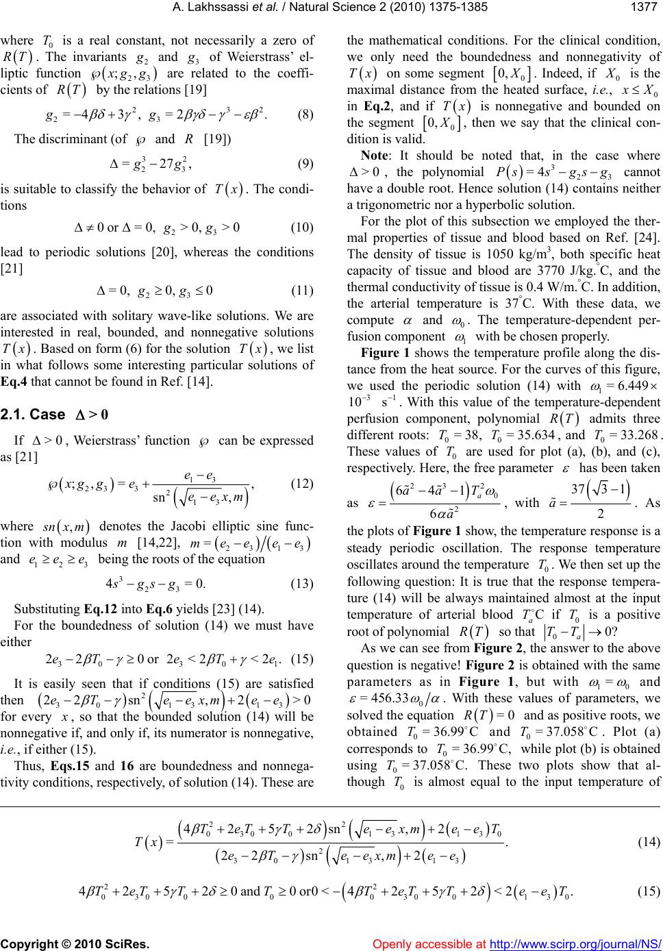 A. L Copyright © 2010 SciRes. Openly accessible at http://www.scirp.org/journal/NS/ akhssassi et al. / Natural Science 2 (2010) 1375-1385 137 1377 where is a real constant, not necessarily a zero of e invariants 0 T . Th RT 2 and 3 of Weierstrass’ el- tion liptic func 23 ;, gg e rela by thtiare related to the coeffi- ons [ 2 cients of RT 19] 23 23 =43,=2.gg (8) The discrimi nant (of and [19]) R 32 23 =27, g (9) is suitable to classavior of Tx. The condi- tions ify the beh lead s nditions [2 solut d in real, bounded, and nonnegative solutions . Based on form (6) for the solution 2.1. Case 23 0or =0,>0,>0gg (10) to periodic solution[20], whereas the co 1] 23 =0, 0,gg0 (11) are associated with solitary wave-like ions. We are intereste Tx Tx, we list in what follows some interesting particular solutions of Eq.4 that cannot be found in Ref. [14]. >0 If >0, Weierstrass’ function can be expressed as [21] 13 23 3213 ;, =, sn , ee xg geeexm (12) where , nx n tion with modul m deotes the Jacobi elliptic sine func- us [14,22], m 23 13 =mee ee an h 0. (13) Substituting Eq.12 into Eq.6 yield s [23] (14 For the boundedness of solution (14) we must have 1 .e d 3 e being the roots of te equation 12 ee 323 4=sgsg ). either 30 3 22 0or2<eTe 0 2 <2T ) It is easily seen that if conditions (15) are s (15 atisfied then 13 , 2>0mee 2 0 13 22 sne Teex for every 3 , so that the bounded so noative, i.e Eqs.15 and 16 are boundedness and nonnega- tivity conditions, resp ectively, of solution (14). The the mathematical conditions. For the clinical condition, we only need the boundedness and nonnegativity of lution (14) will be nnegative if, and on ly if, its numerator is nonneg ., if either (15). Thus, se are Tx on some segment 0 0, . Indeed, if 0 is the al distance fromurface, maxim the heated si.e., 0 X in Eq.2, and if Tx is nonnegative ent and bounded on the segm 0 0, , then we say that the clinical con- is vaditionlid. Note: It should be noted that, in the case where >0 , the polynomial 323 =4Pssgs g cannot ha double root. Hence solution (14) contains neither a trigonometric nor a hyperbolic so lution. For the plot of thissubsection we employed the ther- mal properties of tsue and blood based on Ref. [24]. The density of e is 1050 kg/m3, both specific heat ca ve a is tissu ° th ue is 0 W/m.C. In ° pacity of tissue and blood are 3770 J/kg.C, and the ermal conductivity of tiss.4°addition, the arterial temperature is 37C. With these data, we compute and 0 . The temperature-dependent per- fusion component 1 with be chosen properly. Figure 1 shows the temperature profile along the dis- tance from the heat source. For the curv es of this figu re, we used the periodic solution (14) with 1=6.449 3 10 1 s . With this value of the temperature-dependent perfusion component, polynomial RT admits three different roots: 0=38T, 0= 35.634T, and 0= 33.268T. These values of Tare used for plot (a), (b), and (c), res 0 pectively. Here, the free parameter has been taken as 23 2 0 2 641 6 a aa T a , with 373 1 2 a the plots of Figure 1 show, the temperature response is a steady periodic oscillation. The reponse temperature oscillates around th temperature 0 T. We then set up the following question: It is true that the response tempera- ture (14) will be always maintained almost . As s e at the input perature of arterial blood if is a positiv t of polynomial temC a Te roo 0 T RT so that 00? t a TT As we can see from Figure 2, the answer to the above question is negative! Figure 2 is obtained with the same parameters as in Figure 1, bu with 10 = and 0 =456.33 . With these values of parameters, we solved the equatio n =0RT and as p ositive roots, we obtain ed 0= 36.99CT and CT. Plot (a) corresponds to 0= C,T whilained us 0= 37.058 e plot (36.99 b) is obt ing 0=37.058C.T These two plots show that al- though 0 T is almost equal to the input temperature of 22 0 13 sn 2 e e ee 030 0 2 30 4252 = 22 sn TeT T Tx e T 13 13 13 ,2. , eexm eT exm (14) 2 030 0130 42<2 .T eeT (15) 2 030 00 42520and0or0<TeT TT 25eT T 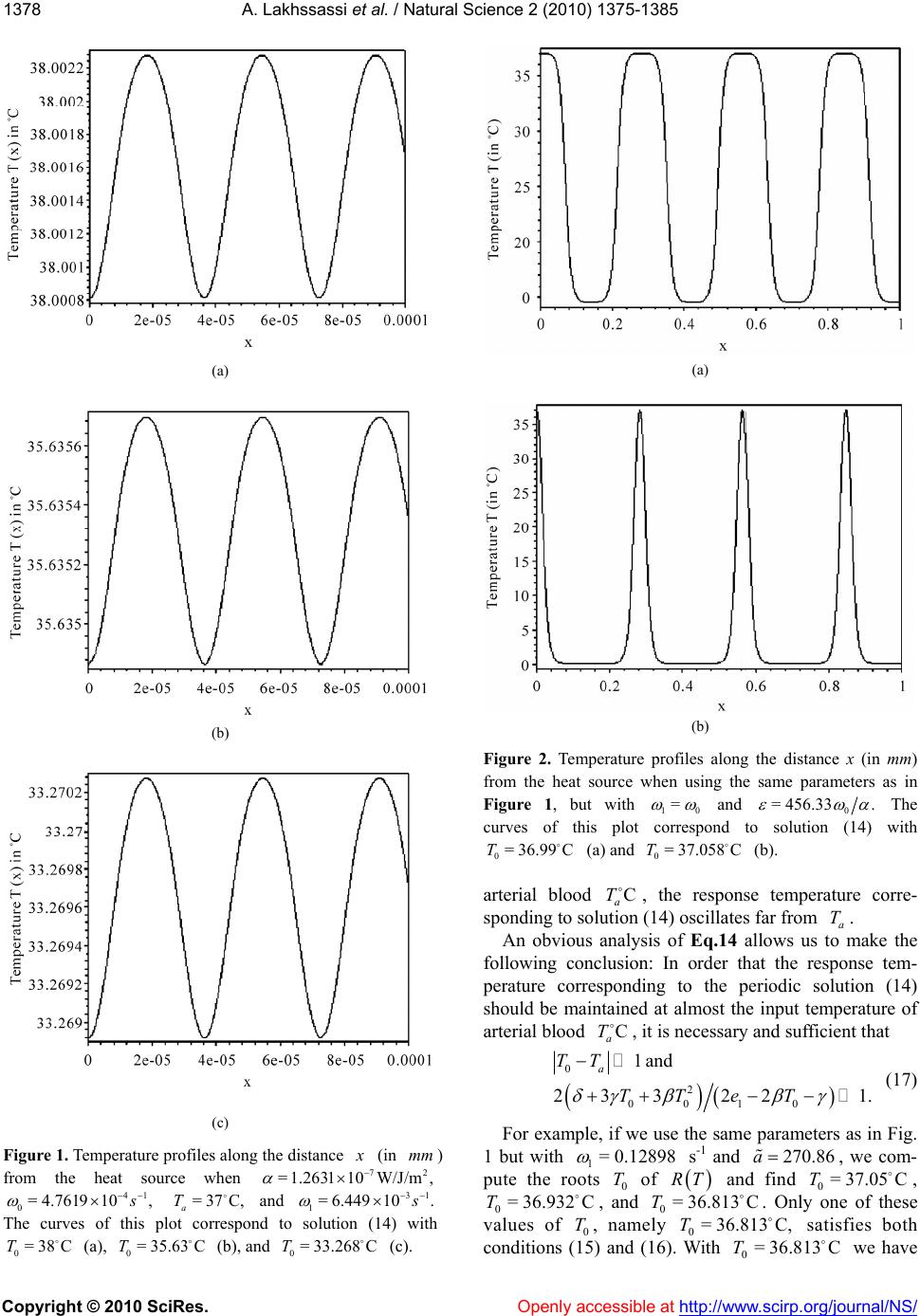 A. L Copyright © 2010 SciRes. Openly accessible at http://www.scirp.org/journal/NS/ akhssassi et al. / Natural Science 2 (2010) 1375-1385 1378 (a) (b) (c) Figure 1. Temperature profiles along the distance (a) (b) Figure 2. Temperature profiles along the distance x (in mm) from the heat source when using the same parameters as in Figure 1, but with 10 = and 0 = 456.33. The curves of this plot nd to solution (14) with (a) and (b). arterial blood , the response temperature corre- sponding to so14) oscillates far from An obviousis of Eq.14 allows usake the following conclusion: In order that the response tem- perature corresponding to the periodic solution (14) should be maintained at almost the input temperature of arterial blood , it is necessary and sufficient that correspo 0= 37.058T 0= 36.99CT C C a T lution ( analysa T. to m C a T 0 2 0010 1and 23 322 a TT TTeT 1. (17) For example, if we use the same parameters as in Fig. 1 but with 1= 0.12898 s -1 and , we com- pute the roo270.86a ts 0 T of RT 36.81 0= 3 With (in ) from the heat source when mm 72 /J/m, =1.2631W 10 41 0= 4.761910, =37C, a T and 1= 61031 ..449 with (c). espond to solu and 0= 33.268T The curves of this p 0=38CT (a), 0=T lot corr 35.63 C (b), tion (14) C and find 0 T C. Only one 813 C, satisf 0= 36.813C =37.05C , of these ies both we have 0= 36.932T values of conditions (1 C , and 0=T 0 T, namely T 5) and (16). 3 6. T 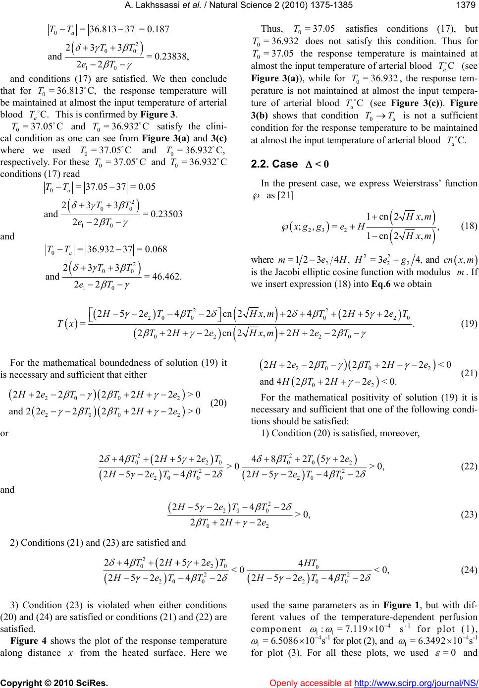 A. Lakhssassi et al. / Natural Science 2 (2010) 1375-1385 Copyright © 2010 SciRes. Openly accessible at http://www.scirp.org/journal/NS/ 137 1379 0 2 00 10 =36.81337= 0.187 23 3 and= 0.23838, 22 a TT TT eT and conditions (17) are satisfied. We then conclude that for the response temperature will be maine input temperature of arterial blood irmed by Figur e 3. satisfy the clini- ure 3(a) and 3(c) ed h and co read 0= 36.813C,T tained at almost th C. a This is conf 37.05 C and T T = 0 T cal condition as on where we us respectively. For t nditions (17) 0= 36.932C e can see from Fig = 37.05C and 0=37.05CT 0 T ese 0= 36.932C,T 0= 36.932CT 0=37.05= 0.05 a TT 2 00 10 23 3 and= 0.23503 22 TT eT and 37 0=36.93237=0.068 a TT 2 00 23 3TT Thus, satisfies conditions (17), but satisfy this condition.hus for temperature is matained at erature of arterial blood (see r the rem- taine inpupera- gure 3(Figure is noicient e to be mtained rial blood 2.2. Case 10 and =46.462. 22eT 0=37.05T 32 does not the response e input temp a)), while fo re is not main terial blood ows that cond for the resp st the input tem 0=36.9T 0=37.05T almost th 3( peratu ture of ar 3(b) sh condition at almo T in C a T sponse te t tem ). t a suff ain a T Figure 0=36.932T, ed at almost th C a T (see Fi n 0a TT se temperatur erature of arte itio on p c) C. <0 In the present case, we express Weierstrass’ function as [21] 23 2 1cn2 , ;, =1cn2, , xm xg geH xm (18) where 2 =12 34meH , 22 22 =3 4 eg, and ,cnx m us m. If is the Jacobi elliptic cosine function with modul we insert expression (18) into Eq.6 we obtain 2 20 0 02 2524 2cn =222cn 2 0 20 20 2 ,24252. 2,222 eTT Tx TH e HxmT HeT HxmHeT (19) For the mathematical boundedness of solution (19) it is necessary and sufficient that either 02 222222>0HeTT He 20 02 2 0 and 222222> 0eTTHe (20) or 20 02 02 222222<0 and 4222<0. HeTTHe HTH e (21) For the mathematical positivity of solution (19) it is necessary and sufficient that one of the following condi- tions should be satisfied: 1) Condition (20) is satisfied, moreover, 22 020 2 2452 >0 eT 002 2 20 020 0 248252 >0, 2524 22524 2 THTT e H eTTH eTT (22) and 2 20 0 0 22TH 2) Conditions (21) and (23) are satisfied and 2 25242 >0, 2 HeTT e (23) 2 0 24 2TH 2 0 2 20 0 24 2eTT 3) Condition (23) is en eith (20) and (24) are satisfieons (21 satisfied. 02 20 0 52 4 <0 <0, 252524 2 eT HT H HeTT (24) violated wher conditions d or conditi) and (22) are Figure 4 shows the plot of the response temperature along distance from the heated surface. Here we used the same parameters as in Figure 1, but with dif- ferent values of the temperature-dependent perfusion component s -1 for plot (1), 4 11 := 7.11910 4 10 1= 6.5086 s-1 for plot (2), and 4 1=6.3492 10 s we used =0 -1 for plot (3). For all these plots, and 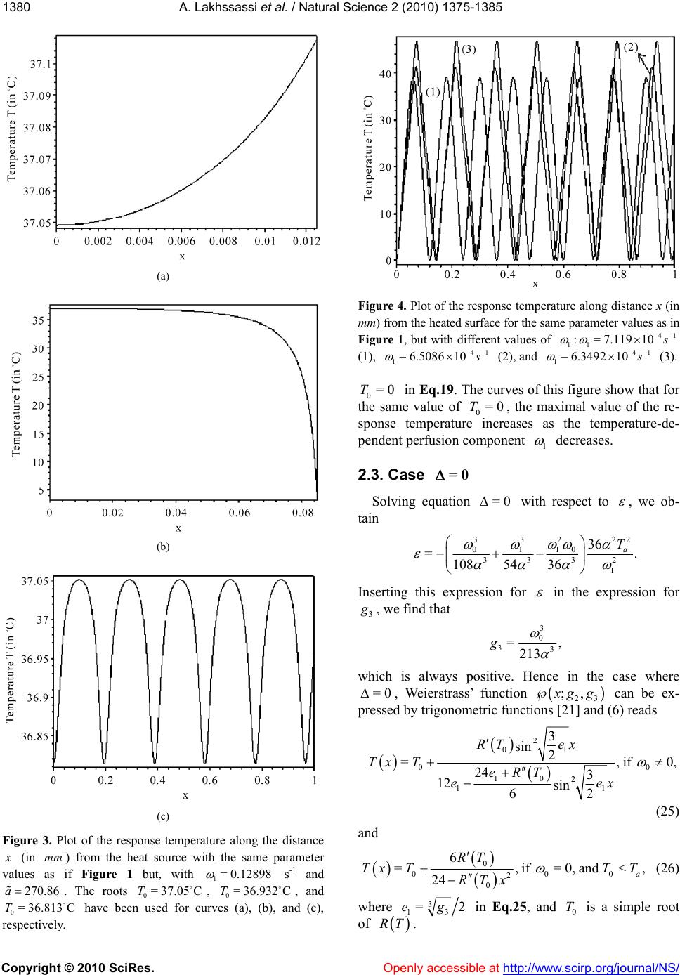 A. Lakhssassi et al. / Natural Science 2 (2010) 1375-1385 Copyright © 2010 SciRes. Openly accessible at http://www.scirp.org/journal/NS/ 1380 (a) (b) (c) Figure 3. Plot of the response temperature along the distance (in ) from the heat source with the same parameter if Figure 1 but, with mm as values1= 0.12898 s -1 and . The roots , and have beenc), 270.86 36.813 ively. a 0 T res 0= 37.05CT used for , 0= 36.932T curves (a), (b),C and (= pect C Figure 4. Plot of the response temperature along distance x (in mm) from the heated surface for the same parameter value Figure 1, but with different values of s as in 41 0 11 := 7.1191 (1), 41 1= 6.508610 (2), and 1= 6.34921041 (3). 0=0T in Eq.19. The curves of this figure show that for the same value of =0T0, the maximal va onse temperature increases as the tem lue of the re- perature-de- perfusion cnt sp pendentompone 1 decreases. 2.3. Case =0 Solving equation =0 with respect to , we ob- tain 3222 336 T 01 0 1 3332 1 =. 108 54 36 a Inserting this expression for in the expression for 3 , we find that 3 0 33 =, 213 g which is always positive. Hence in the case where =0 , Weierstrass’ function 23 ;, gg ions [21] and (can be ex- by trigonometric funct6) reads pressed 2 01 00 10 2 11 3 sin 2 =, 24 3 12 sin 62 RT ex Tx TeRT eex if0, (25) and 0 00 2 0 6 =,if=0,and 24 a RT TxTT T RTx 0 <, (26) here w3 13 =2eg in Eq.2 nd is a simple root 5, a0 T of RT . 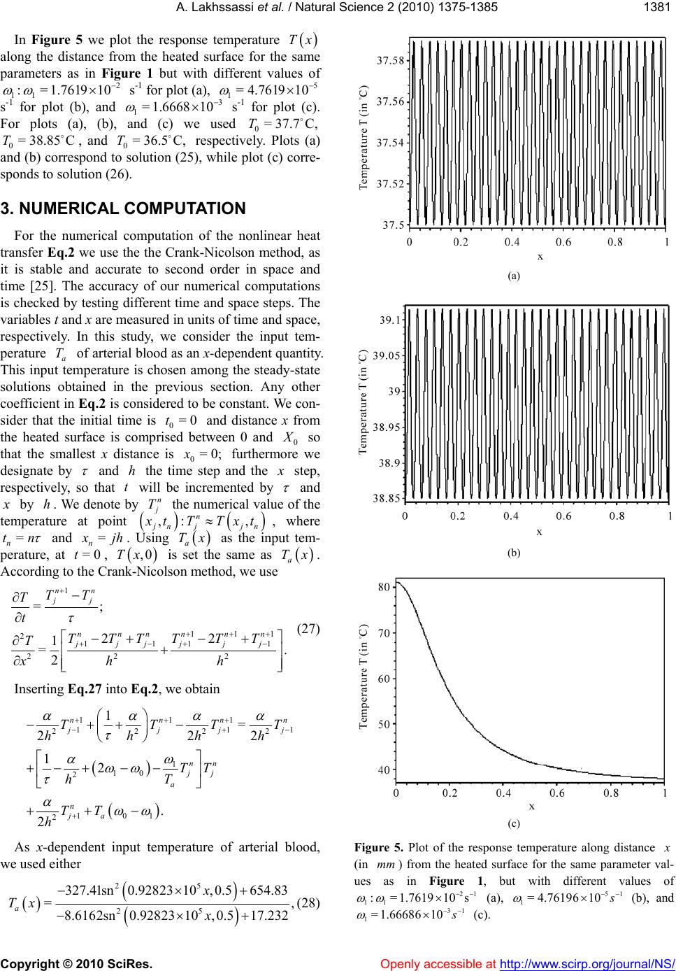 A. Lakhssassi et al. / Natural Science 2 (2010) 1375-1385 Copyright © 2010 SciRes. Openly accessible at http://www.scirp.org/journal/NS/ 138 1381 In Figure 5 we plot the response temperature Tx e same ues of along the distance from the heated surface for th parameters as in Figure 1 but with different val 1 :2 1=1.7619 10 s -1 for plot (a), 5 9 10 1=4.761 plot (c). 37.7 C, Plots (a) orre- s-1 For 0 T and for plot (b), and plots (a), (b), = 38.85C , and 0 T (b) correspond to s 3 s -1 for d 0=T respectively. hile plot (c) c 1=1.666810 and (c) we use =36.5C, olution (25), w sponds to solution (26) . 3. NUMERICAL COMPUTATION For the numerical computation of the nonlinear heat transfer Eq.2 we use the the Crank-Nicolson method, as it is stable and accurate tcond order in space and me [25]. The accuracy of erical computations s checked by testing different time and space steps. The variables t and x are measured in units of time and space, respectively. In this study, we consider the input tem- perature of arterial blood as an x-dependent quantity. This inpuerature is chosen among the steady-state solutions ained in the previous section. Any other coefficient i Eq.2 is considered to be constant. We con- sider the initial time is and distance x from the heateurface is compbetween 0 and o se our numti i a T t temp obt n at th d s0=0t rised 0 so that thest x distance furthermwe designate by e small is 0 x=0; ore and h the time step and the step, respectively thatented b, so t will be incremy and bynote h. We de by n T the nu ,: nmerical valthe p poiue of tem erature atnt , nj jn tT Txt, where =tn n and = n jh . Using a Tx as the input tem- perature, at =0t, ,0Tx is set the same as a Tx. According to the Crank-Nicolson method, we use 1 111 1111 2 =; 22 = 2 n jj nn nn nn jjjj jj TT T TTT TT x (27) 2 22 1 n t T T hh Inserting Eq.27 into Eq.2, we obtain . 111 11 2222 1 10 2 101 2 1= 222 12 . 2 nnnn 1 jj j nn jj a n ja TTTT hhhh TT T h TT h As x-dependent input temperature of arterial blood, we used either 25 25 327.41sn0.92823 10,0.5654.83 =, 8.6162sn0.92823 10,0.517.232 a x Tx x (28) (a) (b) (c) distanceFigure 5. Plot of the response temperature along (in mm) from the heated surface for the same parameter val- ues as in Figure 1, but with different values of 21 11 :=1.7619 10 s (a), 51 1=4.7619610 (b), and 31 1=1.66686 10 (c). 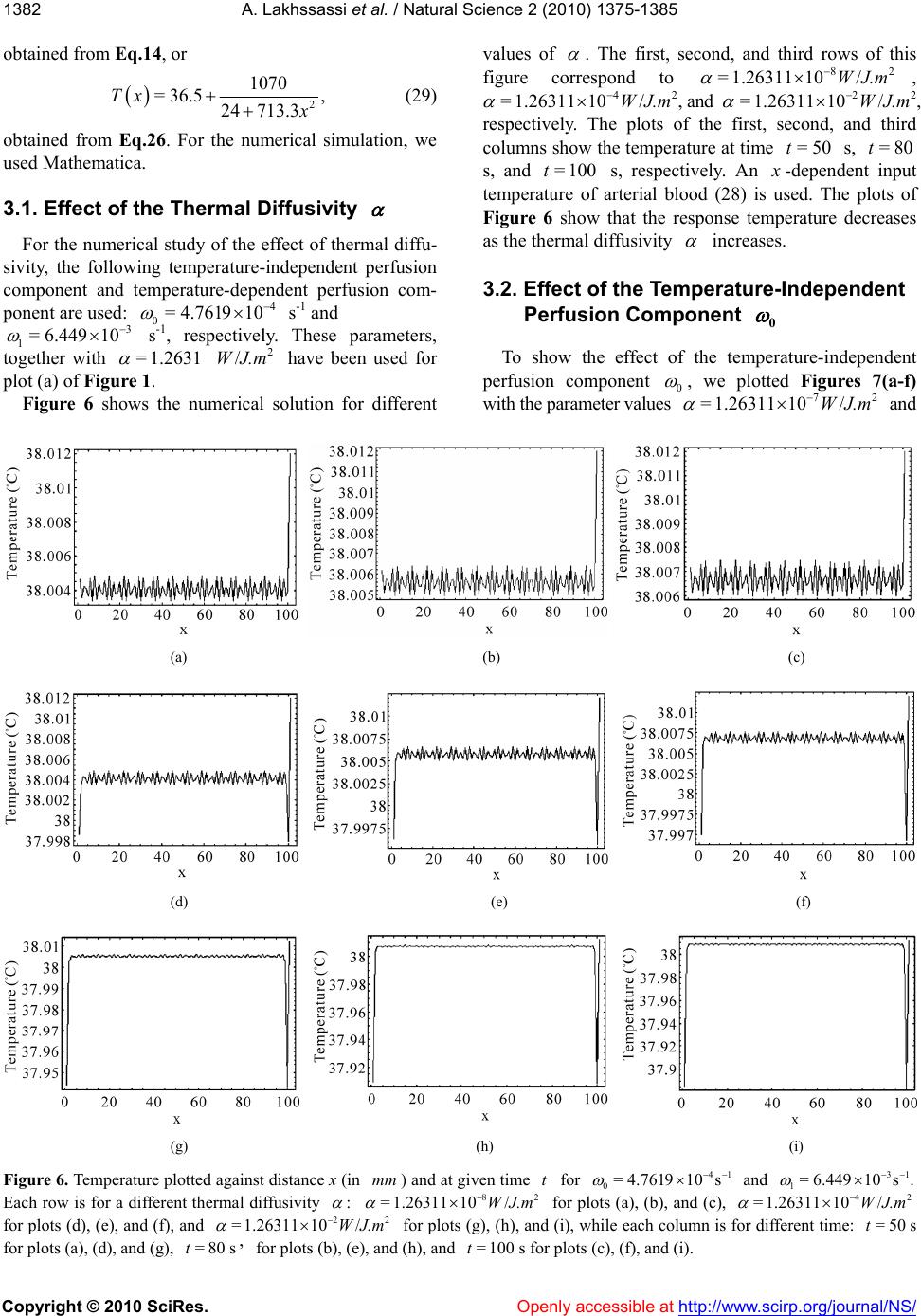 A. Lakhssassi et al. / Natural Science 2 (2010) 1375-1385 Copyright © 2010 SciRes. http://www.scirp.org/journal/NS/ 1382 obtained fr om Eq.14, or Openly accessible at 2 1070 = 36.5, 24 713.3 Tx (29) obtained from Eq.26. For the numerical simulation, we used Mathematica. 3.1. Effect of the Thermal Diffusivity For the numerical study of the effect of thermal diffu- sivity, the following temperature-independent perfusion component and temperature-dependent perfusion com- ponent are used: 4 0=4.7619 10 s -1 and 3 1= 6.44910 s -1, reeters, together with =1.2631 spectively. These param ve been used for plot (a) of Figu Figure 6 shows the numerical solution for dit 2 /WJ.m ha fferen alues of re 1. v . The first, second, and third rows of this figure copond to , rres 11 82 =1.26311 10/WJ.m 42 =1.263 10/WJ.m , and =1.26311 10/WJ. 22 m s of the first, second, and th erature at time =50t s, =8t ectively. An , ird 0 respectiv The plot columns sthe temp s, and t s, resp ely. how =100 -dependent inpu ood (28) is used. The plots o ponse temperature decrea t f ses temperatuof arterial bl Figure 6ow that the res as the thl diffusivity re sh erma increases. 3.2. Effect of the Temperature-Independent Perfusion Component 0 To show the effect of the teerature-independent perfusion componentmp 0 , we plotted Figures 7(a-f with the parameter valu and ) es 72 .26311 10/WJ.m =1 (a) (b) (c) (d) (e) (f) (g) Figure 6. Temperature plotted against distance x (in ) and at givan (h) (i) en time t for 0=4 d 31 1= 6.449 mm 41 .761910 s 10 s . Each row is for a different thermal diffusivity : /WJ 82 =1 22 .m f , and .26311 10/WJ .m or pts (g (h), and =t for plots for plots (d), (e), and (f), and for plots (a), (d), and (g), ( ile each column is for and (i). a), (b), and (c), 42 =1.26311 10/WJ.m ), (h), and (i), wh different time: =50ts 100s for plots (c), (f), =1.26311 10 8, for plots (b), (e)lo =t0s 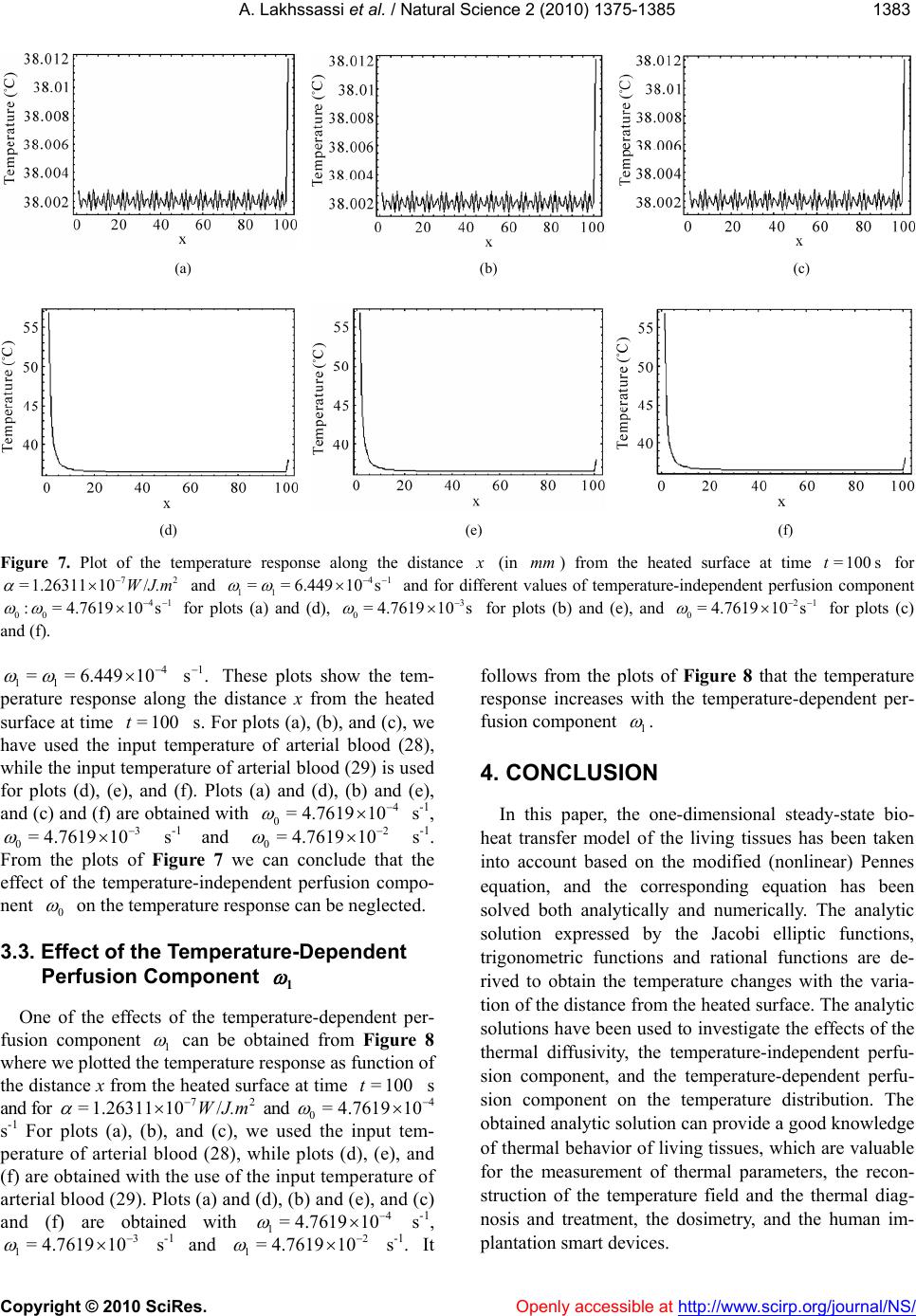 A. Lakhssassi et al. / Natural Science 2 (2010) 1375-1385 Copyright © 2010 SciRes. Openly accessible at http://www.scirp.org/journal/NS/ 138 1383 (a) (b) (c) (d) (e) (f) Figure 7. Plot of the temperature response along the distance (in ) from the heated surface at time for 72 and mm =100st =1.26311 10/WJ.m 41 11 == 6.44910s for plots (a) and (d), 0= 4 and for d of temperature-independent perfuponent for plots (b) and (e), and c) These plots show the tem- distance x from the heated or plots (a), (b), and (c), we ure of arterial blood (28), of arterial blood (29) is used ots (a) and (d), (b) and (e), with iff s erent valuession com for plots ( 41 00 := 4.761910s and (f). 3 .7619 10 21 0= 4.761910s 4 11 == 6.44910 perature response along t surface at time =100t have used the input te while the input temp for plots (d), (e), and ( and (c) and (f) are obtai 1 s. he s. F mperat erature f). Pl ned 4 0=4.7619 10 2 0= 4.761910 s -1, 3 0= 4.761910 s -1 and can conclude that ndent erfusion com s -1. we the ep po- From the plots of Figur effect of the temperature- 0 e 7 ind e p nent on the temperature response can be neglected. 3.3. Effect of the Temperature-Dependent Perfusion Component 1 One of the effects of the temperature-dependent per- fusion component 1 he te 10 can be obtained from Figure 8 where we plotted tmperature response as function of the distance x from the heated surface at time s and for =100t 72 =1.26311 /WJ.m and 4 0= 4.761910 input tem ratu ), and ( 4 10 the - d c) 4.7619 s-1 For pe used peratu lots (a),and (c), w re of arteri ith (b), al blood (28), while plots (d), (e), and (f) are obtained with the use of th e input tempere of arterial blood (29). Plots (a) and (d), (b) an(e and (f) are obtained w1= s -1, 3 1= 4.761910 s -1 2 1= 4.761910 s -1. It and follows from the plots of Figure 8 that the temperature response increases with the temperature-dependent per- fusion component 1 . he o el of on e co b ction e tem ance from been use y, th nd t on th lu ent of t 4. CONCLUSION In this paper, tne-dimensional steady-state bio- heat transfer mod the living tissues has been taken into account based the modified (nonlinear) Pennes equation, and trresponding equation has been he analytic solution expressedy the Jacobi elliptic functions, trigonometric funs and rational functions are de- rived to obtain thperature changes with the varia- tion of the dist the heated surface. The analytic solutions have d to investigate the effects of the thermal diffusivite temperature-independent perfu- sion component, ahe temperature-dependent perfu- sion component e temperature distribution. The obtained analytic sotion can provide a good knowledge are valuable remhermal parameters, the recon- structio and the thermal diag an im plant h solved both analytically and numerically. T of thermal behavior of living tissues, which for the measu n of the temperature field - nosis and treatment, the dosimetry, and the hum- ation smart devices. 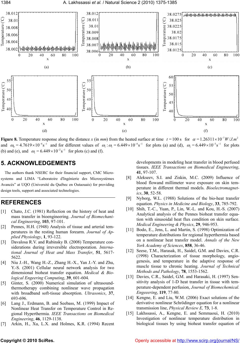 A. Lakhssassi et al. / Natural Science 2 (2010) 1375-1385 Copyright © 2010 SciRes. Openly accessible at http://www.scirp.org/journal/NS/ 1384 (a) (b) (c) (d) (e) (f) Figure 8. Temperature response along the distance x (in mm) from the heated surface at time =100 st for =1.2631 72 1 10/WJ.m and 41 0= 4.761910s and for different values of 4 11 := 6.4410s 1 9 f) for plots (a) and (d), 31 1= 6.44910 plots 21 9 10 . 5. ACKdevelopments in modeling heat trerfused s for (b) andfor plots (c) and ( NOWLEDGEMENTS The authors thank NSERC for n the history of hea ass transfer in. Journal of Biomec lie [3] Davalosa R.V. and Rubinsky B. (2008) Temperature con- a- s [4] ultrasou rmotherapy combining nopagation [7] Arkin, H., Xuolmes, K.R. (1994) ansfer in blood p tissues. IEEE Transactions on Biomedical Engineering, erent thermal models. Bioelectromagnet- ics, 30, 52-58. Solutions of the bio-heat transfer dicine and Biology, 33, 785-792. [1 sing bioheat transfer equation of (e), and 1= 6.44 s their financial support, CMC Micro- systems and LIMA “Laboratoire d'Ingénierie des Microsystèmes Avancés” at UQO (Université du Québec en Outaouais) for providing design tools, support and associated technologies. REFERENCES [1] Chato, J.C. (1981) Reflection ot and m bioengineeringhani- cal Engineering, 103, 97-101. [2] Pennes, H.H. (1948) Analysis of tissue and arterial tem- peratures in the resting human forearm. Journal of Ap- pd Physiology, 1, 93-122. siderations during irreversible electroporation. Intern tional Journal of Heat and Mas Transfer, 51, 5617- 5622. Niu J.-H., Wang H.-Z., Zhang H.-X., Yan J.-Y. and Zhu, Y.-S. (2001) Cellular neural network analysis for two dimensional bioheat transfer equation. Medical & Bio- logical Engeering Computing, 39, 601-604. [5] Ginter, S. (2000) Numerical simulation of nd- the nlinear wave pro with broadband soft-tissue absorption. Ultrasonics, 37, 693-696. [6] Lang J., Erdmann, B. and Seebass, M. (1999) Impact of Nonlinear Heat Transfer on Temperature Control in Re- gional Hyperthermia. IEEE Transactions on Biomedical Engineering, 46, 1129-1138. , L.X. and H Recent 41, 97-107. [8] Alekseev, S.I. and Ziskin, M.C. (2009) Influence of blood flowand millimeter wave exposure on skin tem- perature in diff [9] Nyborg, W.L. (1988) equation. Physics in Me 0] Shih, T.-C., Yuan, P., Lin, W.-L. and Kou, H.-S. (2007) Analytical analysis of the Pennes bioheat transfer equa- tion with sinusoidal heat flux condition on skin surface. Medical Engineering & Physics, 29, 946-953. [11] Bodo, E., Jens, L. and Martin, S. (1998) Optimization of temperature distributions for regional hyperthermia based on a nonlinear heat transfer model. Annals of the New York Academy of Sciences, 858, 36-46. [12] Seese, T.M., Harasak, H., Saidel, G.M. and Davies, C.R. (1998) Characterization of tissue morphology, angio- genesis, and temperature in the adaptive response of muscle tissue to chronic heating. Journal of Technical Methods and Pathology, 78, 1553-1562. [13] Davies, C.R., Saidel, G.M. and Harasaki, H. (1997) Sen- sitivity analysis of 1-D heat transfer in tissue with tem- perature-dependent perfusion, Journal of Biomechemical. Engeeering, 119, 77-80. [14] Kengne, E. and Liu, W.M. (2006) Exact solutions of the derivative nonlinear Schrödinger equation for a nonlinear transmission line, Physical Review E, 73, 1-8. [15] Lakhssassi, A., Kengne, E. and Semmaoui, H. (2010) Investigation of nonlinear temperature distribution in biological tissues by u  A. Lakhssassi et al. / Natural Science 2 (2010) 1375-1385 Copyright © 2010 SciRes. Openly accessible at http://www.scirp.org/journal/NS/ 138 1385 Pennes’type. Journal of Natural Sciences, 2, 131-138. [16] Kengne, E. and Vaillancourt, R. (2009) Exact equilibrium solutions of a diffusion equation with a nonlinear diffu- sion term by means of Jacobian elliptic functions. Inte- gral Transforms and Special Functions, 1, 1-18. [17] Weierstrass K. and Mathematische W.V. (1915) Johnson, New York, 4-16. [18] Whittaker, E.T. and Watson, G.N. (1927) A Course of Modern Analysis, Cambridge University Press, Cam- bridge. [19] Chandrasekharan, Berlin. 0] Schürmann, H.W. and Serov, S.V. (2004) Traveling wave solutions of a generalized modified. Kadomtsev-Petvi- ashvili equation, Journal of Mathematical Physcis, 45, 2181-2187. [21] Abramowitz, M. and Stegun, A.I. (1972) Handbook of Mathematical Functions. 9th edition, Dover Publications, New York. [22] Byrd, P.F. and Friedman, M.D. (1971) Handbook of el- liptic integrals for engineers and scientists. 2nd Edition, Springer-Verlag, Berlin. [23] Schürmann, H.W., Serov, V.S. and Nickel, J. (2006) Su- perposition in nonlinear wave and evolution equations. International Journal of Theoretical Physics, 45, 1057- 1073. [24] Kou, H.S., Shih, T.C. and Lin, W.L. (2003) Effect of the tribution dur- s function based on the porous model. Physics in Medicine and Bi- ology, 48, 1577-1589. [25] Press, W.H., Flannery, B.P., Teukolsky, S.A. and Valler- ling, W.T. (1992) Numerical Recipes in Fortran. Cam- bridge University Press, Cambridge. K. (1985) Elliptic Functions. Springer, directional blood flow on thermal dose dis ing thermal therapy: an application of a Green’ [2
|