Journal of Modern Physics, 2013, 4, 54-65
doi:10.4236/jmp.2013.45B011 Published Online May 2013 (http://www.scirp.org/journal/jmp)
Quantum Isomorphic Shell Model: Multi-Harmonic
Shell Clustering of Nuclei
G. S. Anagnostatos
Institute of Nuclear Physics, National Center for Scientific Research Demokritos, Greece
Received 2013
ABSTRACT
The present multi-harmonic shell clustering of a nucleus is a direct consequence of the fermionic nature of nucleons and
their average sizes. The most probable form and the average size for each proton or neutron shell are here presented by
a specific equilibrium polyhedron of definite size. All such polyhedral shells are closely packed leading to a shell clus-
tering of a nucleus. A harmonic oscillator potential is employed for each shell. All magic and semi-magic numbers, g.s.
single particle and total binding energies, proton, neutron and mass radii of 40Ca, 48Ca, 54Fe, 90Zr, 108Sn, 114Te, 142Nd,, and
208Pb are very successfully predicted.
Keywords: Cluster Models; 40Ca, 48Ca, 54Fe, 90Zr, 108Sn, 114Te, 142Nd, 208Pb, Binding Energies; Coulomb Energies;
Proton; Neutron; Mass Radii; Atomic Fermions
1. Introduction
The present work supports a shell clustering of nuclear
structure by taking advantage mainly of two fundamental
properties of nucleons. The first is the fermionic nature
of nucleons and the second is that nucleons possess finite
average sizes. As will be explained shortly [see a) and b)
below], the first leads to the shell structure of the nucleus
and the second to the average nuclear sizes. These prop-
erties taken together lead to the aforementioned shell
clustering of the nucleus. Indeed:
a) The fermionic nature of nucleons, due to their anti-
symmetric wave function, makes them behave as if a
repulsive force (of unknown nature) is acting among
them. [1]. This repulsive property of nucleons is derived
not only by this antisymmetrization, but also by the re-
pulsive character of the nuclear force itself, considered as
a result of the quark structure of the nucleons. The exis-
tence of this force shifts the nuclear many-body problem
to the problem of finding the equilibria of repulsive par-
ticles on a sphere, like the sphere of a nuclear shell. Ac-
cording to [2], such equilibria are possible only for spe-
cific numbers of particles and when these particles have
most probable positions at the vertices, or middles of
faces, or middles of edges, or simultaneously at these
characteristic points of regular polyhedra or their deriva-
tive polyhedra. Such polyhedra in the present model
stand for the most probable forms of nuclear shells which
- taken in specific sequence, as we will see below – pre-
cisely reproduce the nuclear magic numbers, with no use
of the strong spin-orbit coupling. It is essential to empha-
size here that the structures of these polyhedra precisely
possess the quantization of orbital angular momentum
[3].
b) In addition, the finite average size of nucleons, to-
gether with the above most probable polyhedral structure
of shells, leads to the average sizes of all nuclear shells
and thus of all nuclei. This is obtained by packing the
shells themselves, i.e., each polyhedral shell reaches its
minimum size, that is, the bags of nucleons at its vertices
come in contact with the bags of nucleons at the vertices
of a previous polyhedron.
However, it should be mentioned that the foundation
of the shell structure of the nucleus is offered by other
theories as well, where the antisymmetrization of the
nucleon wave function and the nuclear interaction play
an important role.
The present approach, where the nuclear structure is
qualitatively derived without reference to the in-
ter-particle forces, is applicable not only in nuclear
physics but also in any other branch of physics where
fermions of definite average size are the constituent par-
ticles. Take, for example, cluster physics when the con-
stituent particles are atoms with half-integer spins; thus
they could be considered as atomic fermions. Thus, the
present paper can guide research in other fields, as well
as in nuclear physics.
2. The Model and Applications

G. S. ANAGNOSTATOS 55
2.1. Specification of Most Probable Forms and
Average Sizes of Nuclear Shells
As mentioned in the introduction the fermionic nature of
nucleons and their average sizes lead to the polyhedral
average shell structure of a nucleus. This structure is dif-
ferent for neutrons and protons, since these two kinds of
nucleons are considered as two different sets of particles.
Indeed, this problem for one set or for two different sets
of repulsive particles on a sphere or on concentric
spheres (like the shapes of closed nuclear shells) was
solved by Leech long ago [2]. According to this refer-
ence, each of these two sets should be in equilibrium by
itself on a sphere or on concentric spheres and the result-
ing two structures should be in a new relative equilibrium
as well.
As aforementioned in the introduction, these equilibria
are obtained at the vertices or middles of faces or mid-
dles of edges of regular polyhedra and their derivative
polyhedra. However, when we consider the middles of
faces or the middles of edges of any of the aforemen-
tioned polyhedra, we obtain the vertices of another regu-
lar or semi-regular polyhedron. Thus, we see that it is
sufficient to consider only the vertices of polyhedra.
These polyhedra are the zerohedron, the octahedron, the
hexahedron (cube), the cuboctahedron, the icosahedron,
the dodecahedron, the rhombic cuboctahedron, the ico-
sidodecahedron, and the rhombic triacondahedron with
numbers of vertices 2, 6, 8, 12, 12, 20, 24, 30, and 32,
respectively. These polyhedra can appear more than one
time. Among them three polyhedra can be analysed as two
symmetric, equilibrium structures with smaller numbers
of vertices having together the same central, angular
structure as the initial polyhedron. Namely, the dodeca-
hedron (20 vertices) can be analysed as a cube (8 vertices)
and the remaining (12 vertices), the icosidodecahedron
(30 vertices) can be analysed as an octahedron (6 vertices)
and the remaining (24 vertices), and the rhombic tri-
acondahedron (32 vertices) can be analysed as an icosa-
hedron (12 vertices) and a dodecahedron (20 vertices)
which can further be analysed as above. Recommended
books for a sufficient familiarity with regular and semi-
regular polyhedra are [4, 5], the former being simple and
very instructive and the latter somewhat more sophisti-
cated.
Since both the initial equilibrium polyhedra and the
polyhedra derived by their aforementioned analyses are
candidates to present the most probable forms of nuclear
shells and sub-shells, what is necessary in the following
is to describe how these polyhedra are concentrically and
most symmetrically [6] arranged in space to present nu-
clear shells and sub-shells.
First, we start with the polyhedra with smaller num-
bers of vertices, i.e., with 2, 6, 8, 12, and 20 vertices.
Among them we assign the polyhedra with triangular
faces (corresponding to stable equilibria [2] and having
number of vertices 2, 6, and 12), i.e., the zerohedron, the
octahedron, and the icosahedron, to the first three neu-
tron shells and the remaining polyhedra (corresponding
to unstable equilibria [2] and having number of vertices 2,
8, and 20), i.e., the zerohedron, the hexahedron (cube),
and the dodecahedron, to the first three proton shells (see
Figure 1). This assignment makes each neutron shell
have a corresponding proton shell with the same rota-
tional symmetry, i.e., a neutron zerohedron corresponds
to a proton zerohedron, a neutron octahedron to a proton
hexahedron, and a neutron icosahedron to a proton do-
decahedron. This assignment, in addition, minimizes the
Coulomb energy, since the aforementioned polyhedra for
protons are of a larger size than those assigned for neu-
trons (see Figure 1). This type of correspondence be-
tween neutron and proton shells is valid for the whole
periodic table of nuclei.
Then, their average sizes are determined with respect
to the average size of a proton (rp = 0.860 fm) and that of
a neutron (rn = 0.974 fm), taken as the only universal size
parameters of the model. This happens by packing the
candidate shells themselves and following the instruct-
tions of the next section for all candidate shells in Figure 1
Figure 1. Most probable forms and average sizes of nuclear
shells and sub-shells for nuclei up to Z = 82 and N = 126.

G. S. ANAGNOSTATOS
56
1. In Table 1 the average shells of Figure 1 which are in
contact with each other are given. Specifically, this table
provides what polyhedron is in contact with a previous
one. In general, the prefix Z stands for a proton polyhe-
dron and the prefix N for a neutron polyhedron.
In Figure 1 the dodecahedra, the icosidodecahedra,
and the rhombic triacondahedra are always analysed as
mentioned earlier. These analyses lead to the maximum
compactness. All octahedra and all cubes in the figure
have parallel edges. However, the dodecahedron Z3 has
parallel edges only with the dodecahedron N8 but not
with dodecahedron Z5. The orientation of Z5 is derived
by rotating either Z3 or N8 90° around the z axis. Simi-
larly, the icosahedron N3 has parallel edges only with the
icosahedron N6 but not with icosahedron Z6. The orient-
tation of Z6 is also derived by rotating N3 or N6 90°
around the z axis. Also, the orientation of icosidodecahe-
dron Z8 is derived from that of icosidodecahedron N4 by
considering similar rotation i.e., again 90°. These rota-
tions lead to pairs of similar polyhedra with perpendicu-
lar edges. All these rotations favour the maximum com-
pactness of the polyhedra involved.
It is worth mentioning that the three proton polyhedra
Z4, Z5, and Z6 are the results of analysis of a rhombic
triacondahedron maintaining the same central, angular
structure , as the three neutron polyhedra N6, N7, and N8
are. Each of these two rhombic triacondahedra could be
derived by rotating the one with respect to the other by
90° around the z axis. Similarly, the polyhedra N4 and
N5, and the polyhedra Z7 and Z8 are the results of analy-
sis of two icosidodecahedra with orientations differing by
90°as well. Finally, the polyhedra N9, N10 and N11 are
angularly related polyhedra. Indeed, the middles of edges
of the cube N9 form the cuboctahedron N11 and the
middles of faces of N11 form the rhombic cuboctahedron
N10. In conclusion, each row of neutron or proton poly-
hedra in Figure 1 angularly refers to one and only one
polyhedron which is analysed as shown in the figure. As
mentioned earlier, each row in Figure 1 of neutron (pro-
ton) polyhedra corresponds to an opposite row of proton
(neutron) polyhedra which have the same rotational
symmetry. In geometrical language, polyhedra with the
same rotational symmetry are called reciprocal.
As we can see in Figure 1, the numbers inside brackets
in the block of a polyhedron close to the central vertical
line of the figure, which are equal to the sum of vertices
of all previous polyhedra including this polyhedron, co-
incide with the magic numbers for protons and neutrons,
i.e., 2, 8, 20, 50, 82, and 126. The numbers inside brack-
ets in the remaining blocks of the figure stand for the
semi-magic numbers 28 and 40 for protons, and 62, 70,
90, and 114 for neutrons. The numbers in the blocks of
N4 and Z7 do not form semi-magic numbers since the
corresponding polyhedra are not present in all cases. As
will be understood later, in many cases the octahedra N4
and Z7 remain as part of the structure of the neighbour-
ing icosidodecahedra N5 and Z8, respectively. The
places of their vertices in the neighbouring polyhedron
are marked with h (hole) and form a similar polyhedron,
as happens in all other cases of analyses of polyhedra
mentioned earlier.
The successful reproduction of magic and semi-magic
numbers by the polyhedra of Figure 1 permits a tentative
assignment of quantum states to the polyhedra vertices
standing as average positions of nucleons. One rule is
that quantum sub-shells are always assigned at the vertices
of the same polyhedron. A test of this tentative assign-
ment of quantum states to the vertices of polyhedra will
be made in the section of the quantum mechanical treat-
ment of the model below. In the future, this assignment
will be further and further tested by employing more and
more nuclear observables.
Table 1. Initial and final radii in Fermi of polyhedra whose bags at their vertices are in contact.
Initial Final Final Final
Polyh. Radius Polyh. Radius Polyh. Radius Polyh. Radius
N1 0.974 Z1 1.554 Z2 2.541 N2 2,511
N2 2.511 Z3 3.946 N3 3.568 N5 4.459
Z2 2.541 Z4 4.341
Z3 3.946 Z6 5.5167
N3 3.568 Z5 5.2122
Z4 4.341 N4 5.0372 N7 6.175
N5 4.459 Z7 6.293
N4 5.0372 Z8 6.8712 N10 6.748
Z5 5.2122 N6 6.6713
Z6 5.5167 N8 6.9329
N7 6.175 N9 8.123
N8 6.9329 N11 7.8688

G. S. ANAGNOSTATOS 57
In Figure 1 the high-symmetry equilibrium polyhedra
[2] employed by the model to represent the most prob-
able forms and average sizes of all nuclear shells and
sub-shells up to Z = 82 and N = 126 are given. Specifi-
cally, at the top of each block of the figure the name of
the polyhedron shown in this block (left) and the quan-
tum states of the nucleons accommodated by this poly-
hedron (right) are listed, separately for protons and neu-
trons. In addition at the bottom-left of each block, in a
black square, the numbering of this polyhedron in suc-
cessive order of filling, preceded with the letter Z for
protons and with the letter N for neutrons, is given. Over
this black square the number of the polyhedral vertices,
and the number of the possible unoccupied vertices
characterized as holes, h (symmetrically distributed and
forming an equilibrium polyhedron themselves), are also
given in parentheses. At the bottom-right of each block
the radius of the polyhedron in units Fermi is listed. Over
this radius the cumulative number of vertices of all pre-
vious polyhedra and this polyhedron is also given in
brackets.
The pieces of information given in this section are suf-
ficient, if someone wants to redefine the most probable
forms and the average sizes of equilibrium polyhedra of
Figure 1 employed as the average forms of nuclear shells.
However, if someone just wants to apply the model to
any nuclear observable, it is sufficient to take the poly-
hedra of this figure for granted and not to get involved
with its derivation.
2.2. Radii of Polyhedra and Coordinates of Their
Vertices
Figure 2 is employed to facilitate the present section.
The sphere labelled 1 (with coordinates of its center x0,
y0, z0) stands for an average nucleon position at a vertex
of a polyhedron with known radius R0. The sphere la-
belled 2 (considered in contact with the previous sphere
and with coordinates of each center x, y, z) stands for an
average nucleon position at a vertex of another polyhe-
dron with unknown radius Rx.
Apparently, among the above totally six coordinates
and the distance d12 between the centers of the two spheres
1 and 2, Eq. (1) is valid
(x- x0)2 + (y- y0)2 + (z- z0)2 = d12
2, (1)
On the line O1 we assume the vertex called 1 (with
coordinates x1, y1, z1) of a polyhedron which has the
symmetries of the polyhedron with known radius R0. On
the line O2 we assume the vertex called 2 (with coordi-
nates x2, y2, z2) of a polyhedron which has the symme-
tries of the polyhedron with unknown radius Rx. It is ap-
parent that the coordinates x0, y0, z0 and x, y, z can be
expressed with respect to the coordinates x1, y1, z1 and x2,
y2, z2, and the radii R0 and Rx as follows:
x0 = R0*x1/R1, y0 = R0*y1/ R1, z0 = R0*z1/ R1
x = Rx* x2/ R2, y = Rx* y2/ R2, z = Rx*z2/ R2
R0
2 = x0 2+ y0 2+ z0 2, Rx 2 = x2+y2+z2,
R1
2 = x1 2+y1 2+z1 2, R2 2 = x2 2+y2 2+z2 2 (2)
By substituting the above relationships to Eq.(1) finally
we obtain Eq.(3)
R2x - [(x1x2+y1y2+z1z2)*2 R0/( R1 R2)] Rx
+ [ R0
2- d12 2] = 0 (3)
The quantity d12 takes on the following numerical val-
ues:
d12 = rn + rn = 1.948 fm when two neutron bags are in
contact,
d12 = rn + rp = 1.834 fm when a neutron bag is in con-
tact with a proton bag, and
d12 = 2*<r2>ch = 1.800 fm when two proton bags are in
contact,
where <r2>ch = 0.900 fm is the average proton charge
radius from the literature [7].
By employing Eq.(3) we can determine the radius of
the new polyhedron Rx with respect to the radius of the
known polyhedron R0 and the coordinates x1, y1, z1 and
x2, y2, z2 of the two auxiliary polyhedra employed. These
coordinates for all kinds of polyhedra involved in Figure
1 are given in Table 2 together with corresponding radii
R1 and R2 necessary for the application of Eq.(3).
If Eq. (3) does not have a solution, then there is no
contact between bag 1 of the known polyhedron and bag
2 chosen at a specific vertex of the candidate polyhedron.
Working in same way, we can check whether there is a
contact of bag 1 with bag 2 considered at another vertex
of the same candidate polyhedron. Usually, we can fore-
see which vertex of the polyhedron under investigation is
closer to the chosen vertex of the known polyhedron and
thus one trial is enough. In general, a simple computer
program can easily solve the problem employing all ver-
tices of the candidate polyhedron simultaneously.
As mentioned, the sequences of polyhedra whose bags
at their vertices are in contact with those of previous
polyhedra are given in Table 1. In this table each poly-
hedron used as known polyhedron with radius R0 (called
initial polyhedron) and the derived polyhedron with ra-
dius Rx (called final polyhedron) are shown together with
their radii. The radius Rx is derived by taking the polyhe-
dron of the same row in the table as initial one and ap-
plying Eqs.(1-3). As shown in the table there are cases
where one specific polyhedron used as an initial polyhe-
dron leads to the derivation of two or three final poly-
hedra of different symmetry. The described procedure
strictly leads to the maximum possible density of poly-
hedra standing as the most probable forms and average
sizes of shells and sub-shells for fermions. No overlap-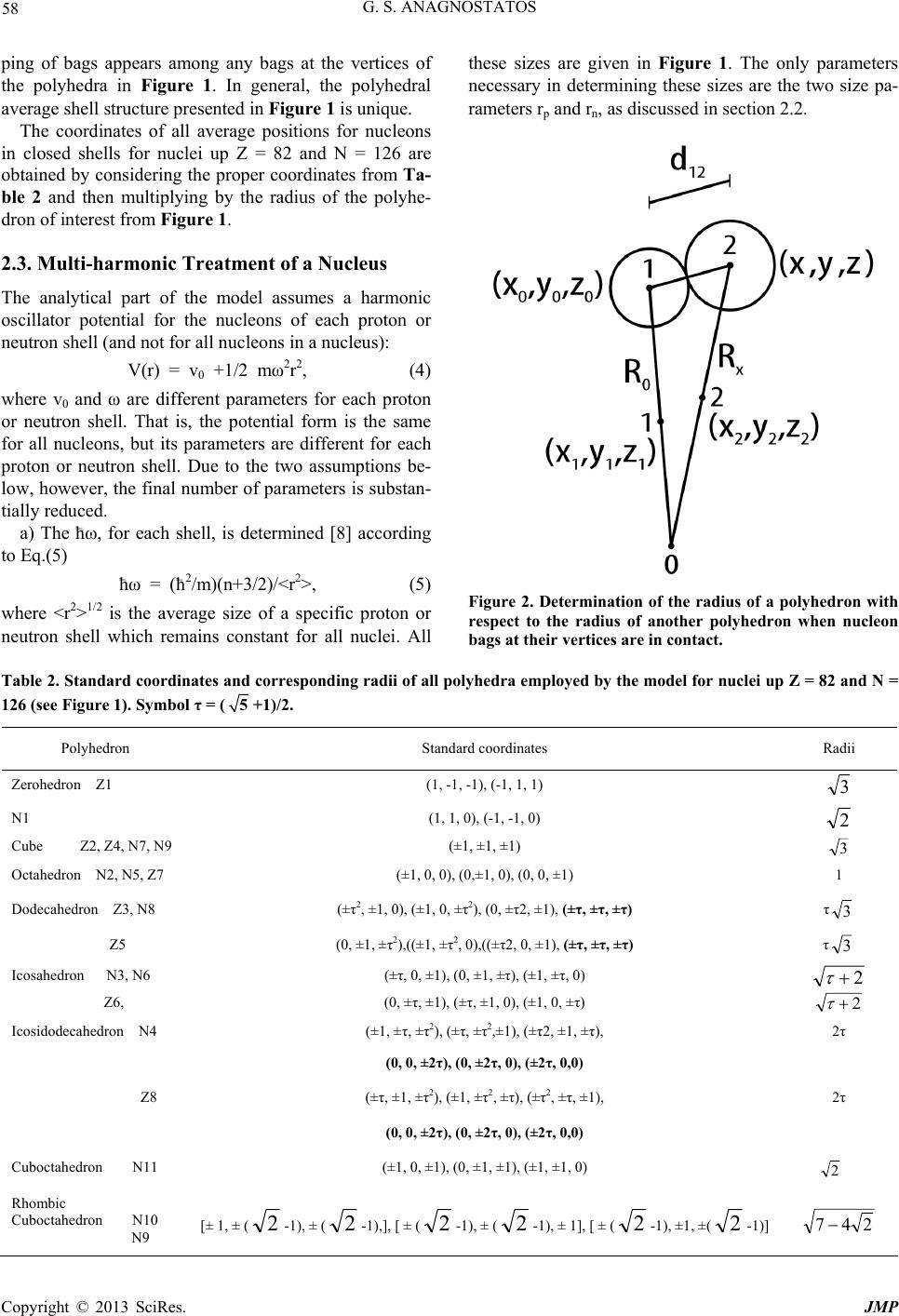

G. S. ANAGNOSTATOS
58
ping of bags appears among any bags at the vertices of
the polyhedra in Figure 1. In general, the polyhedral
average shell structure presented in Figure 1 is unique.
The coordinates of all average positions for nucleons
in closed shells for nuclei up Z = 82 and N = 126 are
obtained by considering the proper coordinates from Ta-
ble 2 and then multiplying by the radius of the polyhe-
dron of interest from Figure 1.
2.3. Multi-harmonic Treatment of a Nucleus
The analytical part of the model assumes a harmonic
oscillator potential for the nucleons of each proton or
neutron shell (and not for all nucleons in a nucleus):
V(r) = v0 +1/2 mω2r2, (4)
where v0 and ω are different parameters for each proton
or neutron shell. That is, the potential form is the same
for all nucleons, but its parameters are different for each
proton or neutron shell. Due to the two assumptions be-
low, however, the final number of parameters is substan-
tially reduced.
a) The ћω, for each shell, is determined [8] according
to Eq.(5)
ћω = (ћ2/m)(n+3/2)/<r2>, (5)
where <r2>1/2 is the average size of a specific proton or
neutron shell which remains constant for all nuclei. All
these sizes are given in Figure 1. The only parameters
necessary in determining these sizes are the two size pa-
rameters rp and rn, as discussed in section 2.2.
Figure 2. Determination of the radius of a polyhedron with
respect to the radius of another polyhedron when nucleon
bags at their vertices are in contact.
Table 2. Standard coordinates and corresponding radii of all polyhedra employed by the model for nuclei up Z = 82 and N =
126 (see Figure 1). Symbol τ = (5+1)/2.
Polyhedron Standard coordinates Radii
Zerohedron Z1 (1, -1, -1), (-1, 1, 1) 3
N1 (1, 1, 0), (-1, -1, 0) 2
Cube Z2, Z4, N7, N9 (±1, ±1, ±1) 3
Octahedron N2, N5, Z7 (±1, 0, 0), (0,±1, 0), (0, 0, ±1) 1
Dodecahedron Z3, Ν8 (±τ2, ±1, 0), (±1, 0, ±τ2), (0, ±τ2, ±1), (±τ, ±τ, ±τ) τ3
Z5 (0, ±1, ±τ2),((±1, ±τ2, 0),((±τ2, 0, ±1), (±τ, ±τ, ±τ) τ3
Icosahedron N3, Ν6 (±τ, 0, ±1), (0, ±1, ±τ), (±1, ±τ, 0) 2


Ζ6, (0, ±τ, ±1), (±τ, ±1, 0), (±1, 0, ±τ) 2

Icosidodecahedron N4 (±1, ±τ, ±τ2), (±τ, ±τ2,±1), (±τ2, ±1, ±τ), 2τ
(0, 0, ±2τ), (0, ±2τ, 0), (±2τ, 0,0)
Ζ8 (±τ, ±1, ±τ2), (±1, ±τ2, ±τ), (±τ2, ±τ, ±1), 2τ
(0, 0, ±2τ), (0, ±2τ, 0), (±2τ, 0,0)
Cuboctahedron N11 (±1, 0, ±1), (0, ±1, ±1), (±1, ±1, 0) 2
Rhombic
Cuboctahedron N10
N9 [± 1, ± (2-1), ± (2-1),], [ ± (2-1), ± (2-1), ± 1], [ ± (2-1), ±1, ±(2-1)] 247 

G. S. ANAGNOSTATOS 59
b) The parameter of the depth of the potential for
each proton or neutron shell is determined according to
Eq.(6)
Ej = vj - ћωj(nj+3/2) = vi - ћωι(ni + 3/2) = Ei, or
vj = vi – ћωi(ni + 3/2) + ћωj(nj+3/2) = V0 + ћωj(nj + 3/2).
(6)
This assumption implies that all nucleons in a nucleus
are equally bound in their own potentials (excluding
Coulomb and spin-orbit interactions).
It is apparent from Eq.(6) that, since according to the
previous assumption a) all ћω are already determined as
above by applying Eq.(5) with respect only of the two
size parameters rp and rn, the depth vi of the potential for
each shell i can be defined with the knowledge of only
one additional parameter V0 (This is the third universal
parameter of the present model equal to 40.268 MeV).
Solving Schroedinger’s equation for the potential of
Eq.(4), we obtain [8] the following equation
Lk
ℓ+1/2 (z) = {[ Γ(1/2Ν + 1/2 ℓ + 1)]2 / k! Γ(ℓ +3/2)}
1F1(-k ; ℓ + 3/2; z), (7)
where 1F1 (α; c; z) = 1+ (α/c)z + α(α+1)z2/c(c+1) 2!+
α(α+1)(α+2)z3/c(c+1)(c+2)3! +…, with c = ℓ + 3/2, α =
-k, z = 2αr2, and α = mω/2ћ. The series terminates with
the term (-1)k[Γ(c)/Γ(c + k)]zk and the various quantum
numbers involved are n = 0,1,2,…; k = 0,1,2,…; k ≤ n/2,
ℓ = 0,1,2,…, ℓ ≤ n, and ℓ = n - 2k [8].
The explicit forms of the first few equations of the
wave functions for a harmonic oscillator potential de-
rived from Eq.(7) can be found in several books of Quan-
tum Mechanics and Nuclear Physics [8]. However, it is
considered instructive for a complete list of all wave
functions for nuclei up to Z = 126 and N = 184, derived
from the recursion formula Eq.(7), to be shown below.
R1s = (128/π)1/4α3/4
2
ar
e
R2s = (128/ π)1/4(3/2)1/2 α3/4 (1- 4αr2/3)
2
ar
e
R3s = (128/π)1/4(15/8)1/2α3/4(1- 8αr2/3 + 16α2r4/15)
2
ar
e
R4s = (128/π)1/4 (35/16)1/2 α3/4 (1- 4αr2 + 16α2r4/5
– 64α3r6/105))
2
ar
e
R1p = (128/π)1/4(4/3)1/2 α5/4 r
2
ar
e
R2p = (128/π)1/4(10/3)1/2 α5/4 r (1 – 4αr2/5)
2
ar
e
R3p = (128/π)1/4 (70/12)1/2 α5/4 r (1 – 8α r2/5
+ 16 α2r4/35)
2
ar
e
R1d = (128/π)1/4 (16/15)1/2 α7/4 r2
2
ar
e
R2d = (128/π)1/4(56/15)1/2 α7/4 r2 (1 – 4α r2/7)
2
ar
e
R3d = (128/π)1/4(252/30)1/2 α7/4 r2 (1 – 8α r2/7
+ 16α2r4/63)
2
ar
e
R1f = (128/π)1/4(64/105)1/2 α9/4 r3
2
ar
e
R2f = (128/π)1/4(288/105)1/2 α9/4 r3 (1 – 4α r2/9)
2
ar
e
R1g = (128/π)1/4(256/945)1/2 α11/4 r4
2
ar
e
R2g = (128/π)1/4(1408/945)1/2α11/4 r4 (1 – 4α r2/11)
2
ar
e
R1h = (128/π)1/4(1024/10395) 1/2 α13/4 r5
2
ar
e
2
R1i = (128/π)1/4(4096/135135 )1/2 α15/4 r6
ar
e
R1j = (128/π)1/4 (16384/2027025)1/2 α17/4 r7 (8)
2
ar
e
As a test, all above wave functions have been checked
for orthonormality.
Due to the fact that in the model ћω is different for the
different shells, the wave functions with the same orbital
angular momentum quantum number ℓ are not orthogo-
nal. For these wave functions Gram-Smidth’s technique
is applied [9].
It is considered instructive to give some relevant guide
equations below to facilitate this orthogonalization.
E2(α1, α2, r) = N2(α1, α2) [R2(α2, r) + b21(α1, α2) R1 (α1, r)]
E3(α1, α2, α3, r) = N3(α1, α2, α3) [R3(α3, r)
+ b32(α1, α2, α3) E2(α1, α2, r)
+ b31(α1, α3) R1(α1, r)]
E4(α1, α2, α3, α4, r) = N4(α1, α2, α3, α4) [R4(α4, r)
+ b
43(α1, α2, α3, α4) E3(α1, α2, α3, r)
+ b42(α1, α2. α4) E2(α1, α2, r)
+ b41(α1, α4) R1(α1, r)], (9)
where
N2(α1, α2) = [1 - b (α1, α2) ]-1/2
2
21
N3(α1, α2, α3) = [1 -b( α1, α2, α3) - b( α1, α3)]-1/2
2
32
2
31
N4(α1, α2, α3, α4)
= [1-b( α1, α2, α3, α4)- b( α1, α2, α4) - b( α1,α4)]-1/2,
2
43
2
42
2
41
(10)
and
b21(α1, α2) = - R1(α1, r) R2(α2, r) r2dr

0
b32(α1, α2, α3) = - E
2(α1, α2, r) R3(α3, r) r2dr

0
b31(α1, α3) = -R1(α1, r) R3(α3, r) r2dr

0
b43(α1, α2, α3, α4) = - E
3(α1, α2, α3, r) R4(α4, r) r2dr

0
b42(α1, α2, α4) = - E2(α1, α2, r) R4(α4, r) r2dr

0
b41(α1, α4) = - R1(α1, r) R4(α4, r) r2dr (11)

0

G. S. ANAGNOSTATOS
60
Also, due to the fact that the model requires the or-
thogonalized wave functions to reproduce the relevant
average radii of polyhedral shells given in Fig.1, some
additional instructive equations are also given below for
radii.
<r2>2 (α1, α2) = E (α1, α2, r) r4dr

0 2
2
<r2>3(α1, α2, α3) = E (α1, α2, α3, r) r4dr

0 2
3
<r2>4(α1, α2, α3, α4) = E (α1, α2, α3, α4, r) r4dr

0 2
4
(12)
While is known that α1 = (m/2ћ2)*ћω1, in the case of
wave functions which need orthogonalization α2, α3, and
α4 in the model are determined as follows. For example
for the case of 2p state for neutrons, while α1 is deter-
mined from Eq.(5) by using the radius 3.568 fm (see N3
in Figure 1), the parameter α2 in the first equation of
(12) must take on a value which leads to the radius
5.0372 fm (see N4 in Figure 1). For the case of 3p state
for neutrons, the parameters α1 and α2 in the second equa-
tion of (12) take on the previous values, while α3 must
take on a value which leads to the radius 7.8688 fm (see
N11 in Figure 1).
2.3.1. Binding Energies
As known, the binding energy for each quantum state in
a harmonic oscillator potential is given by Eq.(13):
EB = v – ћω (n + 3/2). (13)
As aforementioned, in Eq.(13) all ћω come from Eq.(5)
(with respect to the only two size parameters rp and rn)
and all potential depths v come from Eq.(6) (with respect
to the only one additional, potential parameter V0). Thus,
EB from Eq.(13) is determined with respect to only 3
universal parameters.
Now, since the nuclear problem basically refers to
two-body forces, in order to avoid the double counting,
the potential portion of the second part of Eq.(13) should
be divided by two. Further, since according to the Virial
theorem half of the quantity ћω (n + 3/2) is potential en-
ergy and half is kinetic energy, Eq.(13) takes the form of
Eq.(14)
EB =1/2 [v –1/2 ћω (n + 3/2)] - 1/2 ћω (n + 3/2)])
= ½ v – 3/4 ћω (n + 3/2) (14)
Given that the potential v, according to Eq.(6), is
v = V0 + ћω (n + 3/2), (15)
the final expression of binding energy for each proton or
neutron state takes the form of Eq.(16).
(EB)1 = ½ [V0 + ћω (n + 3/2] - 3/4 ћω (n + 3/2)
= ½ V0 – 1/4 ћω1 (n1 + 3/2) (16)
The index 1 in Eq.(16) refers to all states where the
orbital angular momentum quantum number ℓ appears
for the first time.
However, for a second, a third and a fourth appearance
of a state with the same ℓ, in the place of the quantity ћω
(n + 3/2) in Eq.(16) we should take the corresponding
quantity due to the necessary orthogonalization. Thus,
based on Eqs. (9) – (11), we get
(EB)2 = ½ V0 - ¼ N2 [ ћω2*(n2 + 3/2)
+ b21*ћω1(n1 + 3/2)]
(EB)3 = ½ V0 - ¼ N3 {ћω3*(n3 + 3/2)
+ b32*4 [-(EB)2 + ½ V0] + b31*ћω1(n1 + 3/2)}
(EB)4 = ½ V0 - ¼ N4 {ћω4*(n4 + 3/2)
+ b43*4 [-(EB)3 + ½ V0]
+ b42*4 [-(EB)2 + ½ V0] + b41*ћω1(n1 + 3/2)}
(17)
Finally, the total binding energy of a nucleus in the
model is given by Eq.(18)
(EB)total = Σ (EB)i + ΣVLiSi - ΣECij , (18)
A
i1A i1Zji
where: the spin-orbit term is given [8] by Eq.(19)
ΣVLiSi i= λ Σ [i/r*dV(r)/dr]*ℓisi
A
i1A i1
= λ Σ (ћωi)2/(ћ2/m)*ℓisi, (19)
A
i1
with λ = 0.03 (This is the fourth and the last universal
parameter of the present model), and the Coulomb term
is given by Eq.(20):
ΣECij = Σe2/dij. (20)
ZjiZji
The distance dij between any two proton average posi-
tions in Figure 1 is calculated from the coordinates of
the proton polyhedral vertices (standing for the proton
average positions) in this figure (see section 2.2).
An extra term in Eq.(18) due to isospin is not needed
since the isospin is here taken care of by the different
average shell structure between protons and neutrons as
apparent from Figrue 1.
In Table 3 the derived energies (including spin-orbit)
for all proton and neutron single-particle states up to
208Pb are given. Specifically, in col.2 of the table for each
state (col.1) the numerical value of energy for protons
and underneath for neutrons are listed. In col. 4 the en-
ergy of all nucleons in a state (col. 3) is given again in
two rows for each state as before. In the remaining cols.
5-11 the energies from col. 4 relevant to 40Ca, 48Ca, 54Fe,
90Zr, 108Sn, 114Te, 142Nd, and 208Pb are repeated. There,
one can also see which states are considered in the
framework of the model occupied by protons and neu-
trons in the structure of these nuclei.
For all seven nuclei examined 16O is taken as a core.
This means that the 16O experimental binding energy

G. S. ANAGNOSTATOS
61
(127.62 MeV) and its Coulomb energy (11.98 MeV de-
rived from the model) are assumed known. That is, the
energy for the 16O core is taken equal to 139.60 MeV and
is listed in the fourth row from the bottom of Table 3. In
the following row of the table the calculated relevant
Coulomb energies in the framework of the model are
given and underneath, the predicted and experimental
binding energies [10]. The agreements between these two
binding energies are apparent and quite striking. This
agreement is further strengthened by the fact that the
model employed uses only four universal parameters.
Namely, these parameters are: The two size parameters rp
= 0.860 fm and rn = 0.974 fm, the one potential parame-
ter V0 = 40.268 MeV, and the one spin-orbit parameter λ
= 0.03.
As obvious from Table 3 the binding energy of any
nucleus examined is obtained by summing up the ener-
gies of the single particle states involved in this nucleus.
This means that the model employed here considers ex-
clusively an independent particle motion for all nucleons.
In other words, the model considers that for each closed
shell we have a complete saturation of nuclear forces.
Table 3. Single particle and total energies in MeV. Bold numbers are discussed in the text.
StateEnergy# Total
40
Ca
48
Ca
54
Fe
90
Zr
108
Sn
114
Te
142
Nd
208
Pb
1d5/12.0356 72.21 72.2172.2172.2172.2172.2172.2172.2172.21
10.25861.5561.5561.55 61.5561.5561.5561.5561.55 61.55
1d3/ 11.878447.5147.5147.5147.5147.5147.5147.5147.5147.51
10.02340.0940.0940.09 40.0940.0940.0940.0940.09 40.09
2s1/12.4762 24.95 24.9524.9524.9524.9524.9524.9524.9524.95
10.60621.2121.2121.21 21.2121.2121.2121.2121.21 21.21
1f7/12.452899.62 -74.7299.62 99.6299.6299.6299.62
11.924 95.3974.21 95.3995.39 95.3995.3995.3995.39
1f5/12.332673.9973.9973.9973.9973.9973.99
11.78770.7270.72 70.7256.7256.72 56.72
2p3/16.2634 65.0565.0565.0565.0565.0565.05
16.28565.1465.14 65.1465.1465.1465.14
2p1/10.162 20.3220.3220.3220.3220.3220.32
16.22732.4532.45 32.4532.4532.4532.45
1g9/9.9041099.04 -99.0499.0499.0499.04
7.89878.9878.98 78.9878.9878.9878.98
1g7/ 9.721877.77 - - -77.77
7.63561.08 - -61.0861.08
2d5/14.373686.24 -30.3591.06 86.24
17.29103.74103.74 103.74103.74103.74
2d3/15.117460.47 - -60.4760.47
17.267 69.0734.54 69.0769.07 69.07
3s1/12.574225.15 - -25.15
10.84221.6821.6821.68 21.68
1h11/10.90912130.91 -130.91
11.084133.01133.01 133.01
1h9/12.60210126.02 -
10.445 104.45104.45
2f7/ -8 -
16.311 130.49130.49
2f5/ -6 -
16.269 97.6197.61
3p3/ -4 -
17.687 70.7570.75
3p1/ -2 - -
17.644 35.2935.29
1i13/ -14 - -
7.436 104.1104.1
16
O core139.61139.61139.61139.61139.61139.61139.61139.61
E
C
-64.81-64.81-105.92-225.8-330.9 -357.53-448.79-769.24
E
B
mod..342.31416.52 471.31782.98915.18961.131185.14 1636.4
E
B
exp.342.06416.01 471.77783.24914.66961.231185.17 1636.5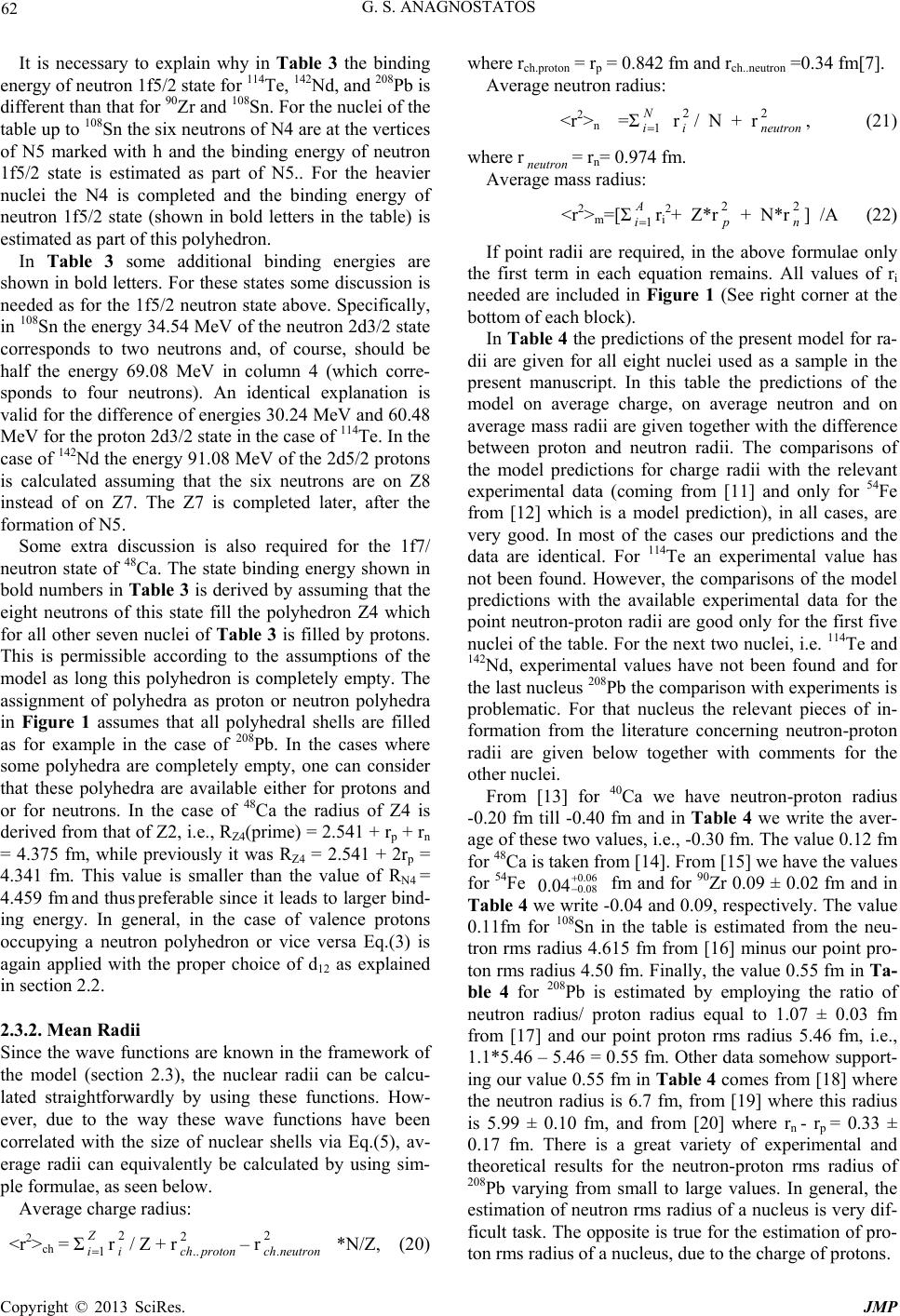

G. S. ANAGNOSTATOS
62
It is necessary to explain why in Table 3 the binding
energy of neutron 1f5/2 state for 114Te, 142Nd, and 208Pb is
different than that for 90Zr and 108Sn. For the nuclei of the
table up to 108Sn the six neutrons of N4 are at the vertices
of N5 marked with h and the binding energy of neutron
1f5/2 state is estimated as part of N5.. For the heavier
nuclei the N4 is completed and the binding energy of
neutron 1f5/2 state (shown in bold letters in the table) is
estimated as part of this polyhedron.
In Table 3 some additional binding energies are
shown in bold letters. For these states some discussion is
needed as for the 1f5/2 neutron state above. Specifically,
in 108Sn the energy 34.54 MeV of the neutron 2d3/2 state
corresponds to two neutrons and, of course, should be
half the energy 69.08 MeV in column 4 (which corre-
sponds to four neutrons). An identical explanation is
valid for the difference of energies 30.24 MeV and 60.48
MeV for the proton 2d3/2 state in the case of 114Te. In the
case of 142Nd the energy 91.08 MeV of the 2d5/2 protons
is calculated assuming that the six neutrons are on Z8
instead of on Z7. The Z7 is completed later, after the
formation of N5.
Some extra discussion is also required for the 1f7/
neutron state of 48Ca. The state binding energy shown in
bold numbers in Table 3 is derived by assuming that the
eight neutrons of this state fill the polyhedron Z4 which
for all other seven nuclei of Table 3 is filled by protons.
This is permissible according to the assumptions of the
model as long this polyhedron is completely empty. The
assignment of polyhedra as proton or neutron polyhedra
in Figure 1 assumes that all polyhedral shells are filled
as for example in the case of 208Pb. In the cases where
some polyhedra are completely empty, one can consider
that these polyhedra are available either for protons and
or for neutrons. In the case of 48Ca the radius of Z4 is
derived from that of Z2, i.e., RZ4(prime) = 2.541 + rp + rn
= 4.375 fm, while previously it was RZ4 = 2.541 + 2rp =
4.341 fm. This value is smaller than the value of RN4 =
4.459 fm and thus preferable since it leads to larger bind-
ing energy. In general, in the case of valence protons
occupying a neutron polyhedron or vice versa Eq.(3) is
again applied with the proper choice of d12 as explained
in section 2.2.
2.3.2. Mean Radii
Since the wave functions are known in the framework of
the model (section 2.3), the nuclear radii can be calcu-
lated straightforwardly by using these functions. How-
ever, due to the way these wave functions have been
correlated with the size of nuclear shells via Eq.(5), av-
erage radii can equivalently be calculated by using sim-
ple formulae, as seen below.
Average charge radius:
<r2>ch = ΣZ
ir/ Z + r– r*N/Z, (20) 1
2
i2 .. protonch 2 .neutronch
where rch.proton = rp = 0.842 fm and rch..neutron =0.34 fm[7].
Average neutron radius:
<r2>n =Σ r2
i/ N + r, (21)
N
i1
2
neutron
where r= rn= 0.974 fm.
neutron
Average mass radius:
<r2>m=[Σri
2+ Z*r + N*r] /A (22)
A
i1
2
p2 n
If point radii are required, in the above formulae only
the first term in each equation remains. All values of ri
needed are included in Figure 1 (See right corner at the
bottom of each block).
In Table 4 the predictions of the present model for ra-
dii are given for all eight nuclei used as a sample in the
present manuscript. In this table the predictions of the
model on average charge, on average neutron and on
average mass radii are given together with the difference
between proton and neutron radii. The comparisons of
the model predictions for charge radii with the relevant
experimental data (coming from [11] and only for 54Fe
from [12] which is a model prediction), in all cases, are
very good. In most of the cases our predictions and the
data are identical. For 114Te an experimental value has
not been found. However, the comparisons of the model
predictions with the available experimental data for the
point neutron-proton radii are good only for the first five
nuclei of the table. For the next two nuclei, i.e. 114Te and
142Nd, experimental values have not been found and for
the last nucleus 208Pb the comparison with experiments is
problematic. For that nucleus the relevant pieces of in-
formation from the literature concerning neutron-proton
radii are given below together with comments for the
other nuclei.
From [13] for 40Ca we have neutron-proton radius
-0.20 fm till -0.40 fm and in Table 4 we write the aver-
age of these two values, i.e., -0.30 fm. The value 0.12 fm
for 48Ca is taken from [14]. From [15] we have the values
for 54Fe fm and for 90Zr 0.09 ± 0.02 fm and in
Table 4 we write -0.04 and 0.09, respectively. The value
0.11fm for 108Sn in the table is estimated from the neu-
tron rms radius 4.615 fm from [16] minus our point pro-
ton rms radius 4.50 fm. Finally, the value 0.55 fm in Ta-
ble 4 for 208Pb is estimated by employing the ratio of
neutron radius/ proton radius equal to 1.07 ± 0.03 fm
from [17] and our point proton rms radius 5.46 fm, i.e.,
1.1*5.46 – 5.46 = 0.55 fm. Other data somehow support-
ing our value 0.55 fm in Table 4 comes from [18] where
the neutron radius is 6.7 fm, from [19] where this radius
is 5.99 ± 0.10 fm, and from [20] where rn - rp = 0.33 ±
0.17 fm. There is a great variety of experimental and
theoretical results for the neutron-proton rms radius of
208Pb varying from small to large values. In general, the
estimation of neutron rms radius of a nucleus is very dif-
ficult task. The opposite is true for the estimation of pro-
ton rms radius of a nucleus, due to the charge of protons.
0.06
0.08
0.04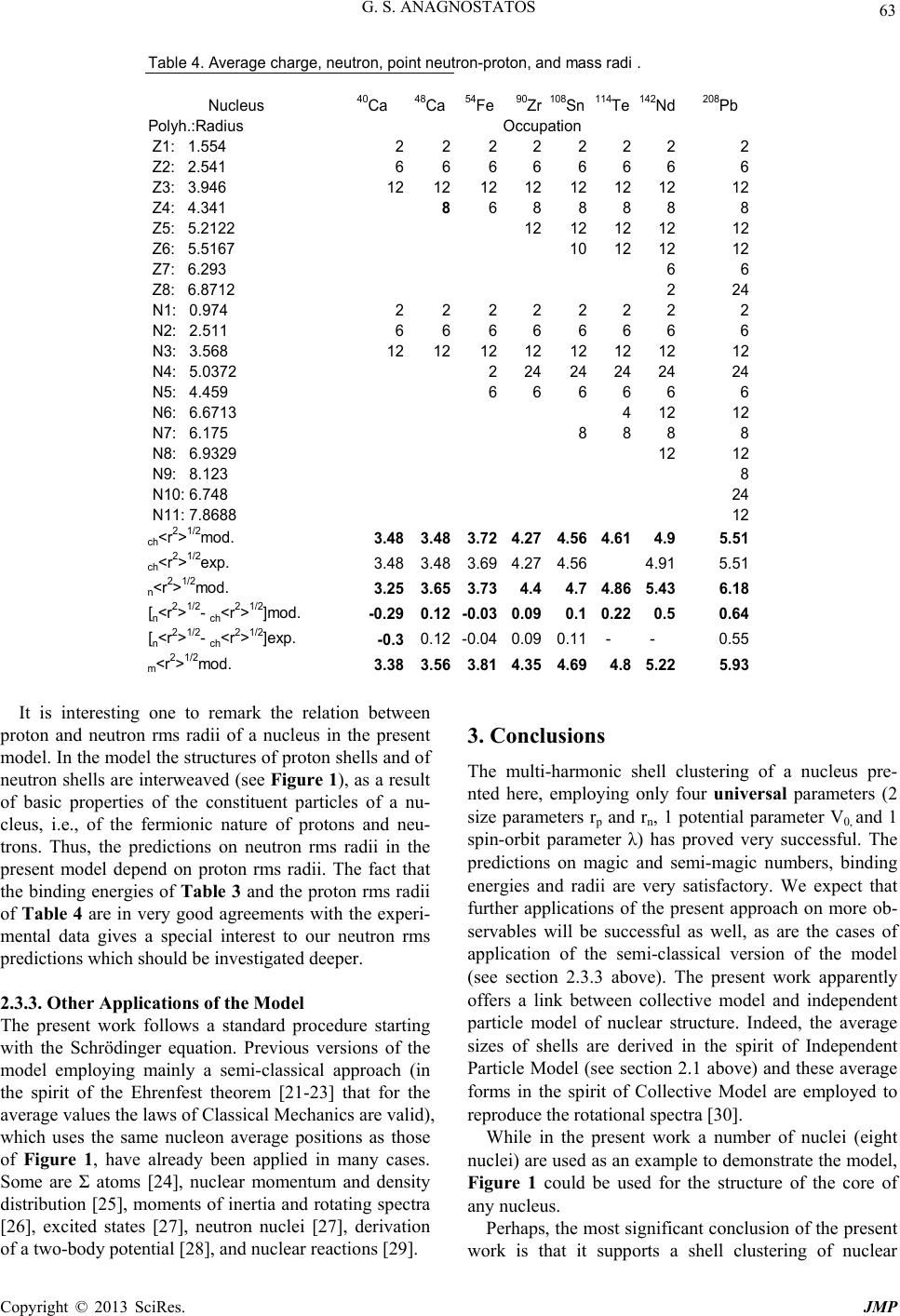


G. S. ANAGNOSTATOS 63
Table 4. Average charge, neutron, point neutron-proton, and mass radi.
Nucleus
40
Ca
48
Ca
54
Fe
90
Zr
108
Sn
114
Te
142
Nd
208
Pb
Polyh.:Radius Occupation
Z1: 1.55422222222
Z2: 2.54166666666
Z3: 3.9461212121212121212
Z4: 4.341868888
Z5: 5.21221212121212
Z6: 5.516710121212
Z7: 6.29366
Z8: 6.8712224
N1: 0.97422222222
N2: 2.51166666666
N3: 3.5681212121212121212
N4: 5.037222424242424
N5: 4.459666666
N6: 6.671341212
N7: 6.1758888
N8: 6.93291212
N9: 8.1238
N10: 6.74824
N11: 7.868812
ch
<r
2
>
1/2
mod. 3.483.483.72 4.274.56 4.614.95.51
ch
<r
2
>
1/2
exp. 3.48 3.48 3.694.274.564.915.51
n
<r
2
>
1/2
mod. 3.253.653.734.44.7 4.86 5.436.18
[
n
<r
2
>
1/2
-
ch
<r
2
>
1/2
]mod. -0.290.12-0.03 0.090.1 0.220.50.64
[
n
<r
2
>
1/2
-
ch
<r
2
>
1/2
]exp. -0.3 0.12-0.040.090.11 - -0.55
m
<r
2
>
1/2
mod. 3.383.563.81 4.354.694.8 5.225.93
8
It is interesting one to remark the relation between
proton and neutron rms radii of a nucleus in the present
model. In the model the structures of proton shells and of
neutron shells are interweaved (see Figure 1), as a result
of basic properties of the constituent particles of a nu-
cleus, i.e., of the fermionic nature of protons and neu-
trons. Thus, the predictions on neutron rms radii in the
present model depend on proton rms radii. The fact that
the binding energies of Table 3 and the proton rms radii
of Table 4 are in very good agreements with the experi-
mental data gives a special interest to our neutron rms
predictions which should be investigated deeper.
2.3.3. Other Applications of the Model
The present work follows a standard procedure starting
with the Schrödinger equation. Previous versions of the
model employing mainly a semi-classical approach (in
the spirit of the Ehrenfest theorem [21-23] that for the
average values the laws of Classical Mechanics are valid),
which uses the same nucleon average positions as those
of Figure 1, have already been applied in many cases.
Some are Σ atoms [24], nuclear momentum and density
distribution [25], moments of inertia and rotating spectra
[26], excited states [27], neutron nuclei [27], derivation
of a two-body potential [28], and nuclear reactions [29].
3. Conclusions
The multi-harmonic shell clustering of a nucleus pre-
nted here, employing only four universal parameters (2
size parameters rp and rn, 1 potential parameter V0, and 1
spin-orbit parameter λ) has proved very successful. The
predictions on magic and semi-magic numbers, binding
energies and radii are very satisfactory. We expect that
further applications of the present approach on more ob-
servables will be successful as well, as are the cases of
application of the semi-classical version of the model
(see section 2.3.3 above). The present work apparently
offers a link between collective model and independent
particle model of nuclear structure. Indeed, the average
sizes of shells are derived in the spirit of Independent
Particle Model (see section 2.1 above) and these average
forms in the spirit of Collective Model are employed to
reproduce the rotational spectra [30].
While in the present work a number of nuclei (eight
nuclei) are used as an example to demonstrate the model,
Figure 1 could be used for the structure of the core of
any nucleus.
Perhaps, the most significant conclusion of the present
work is that it supports a shell clustering of nuclear

G. S. ANAGNOSTATOS
64
structure exclusively based on the fermionic nature of
nucleons and their average sizes. In brief, the anti-sym-
metric wave function of nucleons makes them behave as
if a repulsive force (of unknown nature) is acting among
them. This force for nucleons on spherical shells, in order
to obtain equilibrium of forces (which is a necessary
condition for an independent particle motion of nucleons),
it leads to equilibrium structures for nuclear shells, i.e., to
the structures of regular polyhedra and their derivative
polyhedra [2, 4-5]. Furthermore, these polyhedral struc-
tures are finally closed packed to obtain maximum nu-
clear density for the average positions of nucleons by
taking advantage of their finite sizes.
The basic computer programs employed by the present
work are available on request.
4. Acknowledgements
The author is deeply indebted to Dr. D. Lenis of our In-
stitute for his excellent computer work related to the
present manuscript.
REFERENCES
[1] C. W. Sherwin, “Introduction to Quantum Mechanics,”
Holt Rinehart and Winston, New York, 1959, p.205.
[2] J. Leech, “Equilibrium of Sets of Particles on a Sphere,”
Mathematical Gazette, Vol. 41, No. 36, 1957, pp. 81-90.
doi:10.2307/3610579
[3] G. S. Anagnostatos, “Symmetry Description of the Inde-
pendent Particle Model,” Lettere Al Nuovo Cimento, Vol.
29, No. 6, 1980, pp. 188-192.
[4] G. S. Anagnostatos, “The Geometry of the Quantization
of Angular Momentum (ℓ, s, j) in Fields of Central Sym-
metry, Lettere Al Nuovo Cimento, Vol. 28, No. 17, 1980,
pp. 573- 576.
[5] G. S. Anagnostatos, J. Giapitzakis, A. Kyritsis, “Rota-
tional Invariance of Orbital-Angular-Momentum Quanti-
zation of Direction for Degenerate States”, Lettere Al
Nuovo Cimento, Vol. 32, No. 11, 1981, pp. 332-335.
doi:10.1007/BF02745301
[6] H. M. Cundy and A. P. Rollett, “Mathematical Models,”
2nd Ed., Oxford University Press, 1961, p.76.
[7] H. S. M. Coxeter, “Regular Polytopes”, 2nd Ed., The
Macmillan Company, New York, 1963.
[8] G. S. Anagnostatos, “Isomorphic Shell Model for
Closed-Shell Nuclei, ” International Journal of
Theoretical Physics, Vol. 24, 1985, pp. 579-613.
doi:10.1007/BF00670466
[9] De Jager, C. W. H. de Vries, C. de Vries, “Nuclear
Charge and Momentum Distribution,” Atomic Data and
Nuclear Data Tables, Vol. 14, No. 5-6, 1974, pp. 479-665.
doi:10.1016/S0092-640X(74)80002-1
[10] W. F. Hornyak, “Nuclear Structure,” Academic, New
York, 1975, p 13.
[11] J. D. Vergados, “Mathematical Methods in Physics,”
Akourastos Giannis, Greece, 1970.
[12] A. H. Wapstra and N. B. Gove, “Atomic Mass Table,”
Automic Data and Nuclear Data Tables, Vol. 9, 1971, pp.
267-301.
doi:10.1016/S0092-640X(09)80001-6
[13] E.G.Nadjakov, K.P.Marinova, and Yu.P.Gangrsky, “Sys-
tematics of Nuclear Charge Radii”, Automic Data and
Nuclear Data Tables, Vol. 56, 1994, pp. 133-167.
doi:10.1006/adnd.1994.1004
[14] I. Angeli, “Recommended Values of R.M.S. Charge Ra-
dii”, Heavy Ion Phys., Vol. 8, No. 1-2, 1998, pp. 23-29.
[15] L. Ray, G. W. Hoffmann, and W. R. Coker, “Nonrelativ-
istic and Relativistic Descriptions of Proton-Nucleus
Scattering,” Physics Reports, Vol. 212, No. 5, 1992, pp.
223-328. doi:10.1016/0370-1573(92)90156-T
[16] R. C. Barrett., “Colloques,” Journal de Physique, Vol. 34,
1973, pp. 23-28.
[17] A. Trzcinska, “Nuclear Periphery Studied with Antipro-
tonic Atoms”, Hyp. Inter., Vol. 194, No. 1, 2009, pp.
271-276.
[18] J. Terasaki, J. Engel, “Self-Consistent Description of
Multipole Strength: Systematic Calculations,” Physical
Review C, Vol. 74, No. 4, 2006, pp. 044301-044319.
doi:10.1103/PhysRevC.74.044301
[19] S. D. Schery, D. A. Lind and C. D. Zafiratos, “Radius of
the Neutron Distribution in 208Pb from (p, n) Quasielastic
Scattering,” Physical Review C, Vol. 9, No. 1, 1974, pp.
416-418. doi:10.1103/PhysRevC.9.416
[20] G. F. Bertsch, P. F. Bortignon, R. A. Broglia, “Damping
of Nuclear Excitations,” Reviews of Modern Physics, Vol.
55, 1983, pp. 287-314. doi:10.1103/RevModPhys.55.287
[21] H. J. Koemer and J. P. Schiffer, “Neutron Radius of 208Pb
from Sub-Coulomb Pickup,” Physical Review Letters,
Vol. 27, No. 21, 1971, pp. 1457-1460.
doi:10.1103/PhysRevLett.27.1457
[22] S. Abrahamyan, Z. Ahmed, H. Albataineh, K. Aniol. D. S.
Armstrong, et al., “Measurement of the Neutron Radius
of 208Pb through Parity-Violation in Electron Scattering”,
cited as: arXiv: 1201.2568v2 [nucl-ex], Cornell
University Library, 13 Jan. 2012, journal reference:
Physical Review Letters, Vol. 108, No. 11, 2012, pp.
112502-112507.
[23] E. Merzbacher, “Quantum Mechanics,” John Wiley and
Sons, Inc. New York, 1961, p. 42
[24] C. Cohen-Tannoudji, B. Diu, F. Laloe, “Quantum
Mechanics, ” John Wiley & Sons, New York, 1977, p.
240.
[25] A. Bohr, B. R. Mottelson, “Nuclear Structure,” W. Α.
Benjamin, Inc., Advanced Book Program, Reading, Mas-
sachusetts, London, Vol. 2, 1975.
[26] J. Dabrowski, J. Rozynek and G. S. Anagnostatos, “Σ-
Atoms and the ΣΝ Interaction,” Eur. Phys. J. A, Vol. 14,
2002, pp. 125-131.
[27] G. S. Anagnostatos, A. N. Antonov, P. Ginis, J.
Giapitzakis and M. K. Gaidarov, “Nucleon Μomentum
and Density Distributions in 4He Considering Internal
Rotation,” Physical Review C, Vol. 58, No. 4, 1998, pp.

G. S. ANAGNOSTATOS
65
2115-2119.
[28] M. K. Gaidarov, A. N. Antonov, G. S. Anagnostatos, S. E.
Massen, M. V. Stoitsov and P. E. Hodgson, “Proton Mo-
mentum Distribution in Nuclei beyond 4He,” Physical
Review C, Vol. 52, No. 6, 1995, pp. 3026-3031.
[29] G. S. Anagnostatos, P. Ginis, J. Giapitzakis, “α-Planar
States in 28Si, ” Physical Reviewe C, Vol. 58, No. 6, 1998,
pp. 3305-3315 doi:10.1103/PhysRevC.58.3305
[30] P. K. Kakanis and G. S. Anagnostatos, “Persisting
α-Planar Structure in 20Ne,” Physical Review C, Vol. 54,
No. 6, 1996, pp. 2996-3013.
doi:10.1103/PhysRevC.54.2996
[31] G. S. Anagnostatos, “Classical Equations-of-Motion
Model for High-Energy Heavy-Ion Collisions,” Physical
Review C, Vol. 39, No. 3, 1989, pp. 877-883.
doi:10.1103/PhysRevC.39.877
[32] G. S. Anagnostatos and C. N. Panos, “Semiclassical
Simulation of Finite Nuclei,” Physical Review C, Vol. 42,
No. 3, 1990, pp. 961-965. doi:10.1103/PhysRevC.42.961
[33] G. S. Anagnostatos, “Towards A Unification of Inde-
pendent and Collective Models, 20th Conference of the
Hellenic Nuclear Physical Society, Athens, May 27-28,
2011 (PDF in: www.uoi.gr/HNPS).
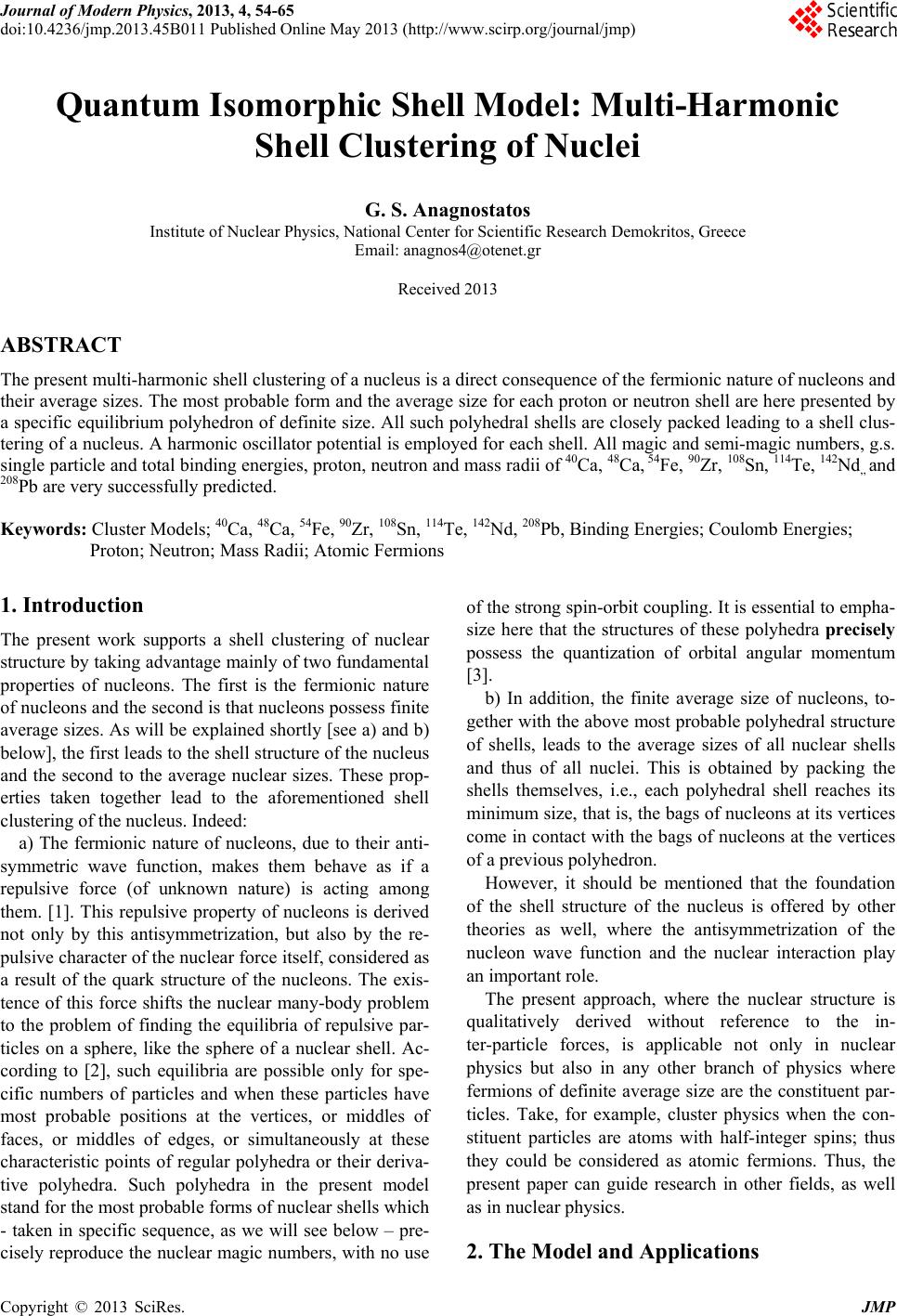