H. D. XU ET AL. 43
output waveform with minimal pedestal recovering time,
which can largely relax the ADC sample rate while re-
taining sufficient samples for post-processing.
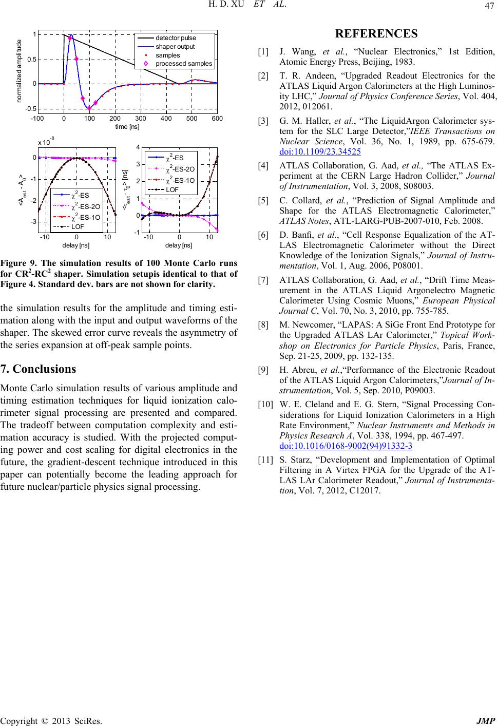
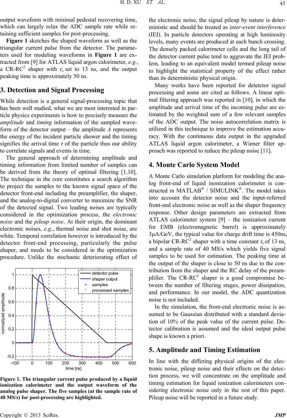
Figure 1 sketches the shaped waveform as well as the
triangular current pulse from the detector. The parame-
ters used for modeling waveforms in Figure 1 are ex-
tracted from [9] for ATLAS liquid argon calorimeter, e.g.,
a CR-RC2 shaper with τs set to 13 ns, and the output
peaking time is approximately 50 ns.
3. Detection and Signal Processing
While detection is a general signal-processing topic that
has been well studied, what we are most interested in par-
ticle physics experiments is how to precisely measure the
amplitude and timing information of the sampled wave-
form of the detector output – the amplitude A represents
the energy of the incident particle shower and the timing
signifies the arrival time τ of the particle thus our ability
to correlate signals and events in time.
The general approach of determining amplitude and
timing information from limited number of samples can
be derived from the theory of optimal filtering [1,10].
The technique in the core constitutes a search algorithm
to project the samples to the known signal space of the
detector front-end including the preamplifier, the shaper,
and the analog-to-digital converter to maximize the SNR
of the detected signal. Two leading noises are typically
considered in the optimization process, the electronic
noise and the pileup noise. At their origin, the dominant
electronic noises, e.g., thermal noise and shot noise, are
white. Temporal correlation however is introduced by the
detector front-end processing, particularly the pulse
shaper, and needs to be considered in the optimization
procedure. Unlike the stochastic deteriorating effect of
-100 0100 200 300 400 500 600
-0.2
0
0.2
0.4
0.6
0.8
1
time [ns]
norm a lized amplitude
det ect or pulse
sha per o utp ut
samples
proce ssed sa m pl es
Figure 1. The triangular current pulse produced by a liquid
ionization calorimeter and the output waveform of the
analog pulse shaper. The five samples (at the sample rate of
40 MS/s) for post-processing are highlighted.
the electronic noise, the signal pileup by nature is deter-
ministic and should be treated as inter-event interference
(IEI). In particle detectors operating at high luminosity
levels, many events are produced at each bunch crossing.
The densely packed calorimeter cells and the long tail of
the detector current pulse tend to aggravate the IEI prob-
lem, leading to an equivalent model termed pileup noise
to highlight the statistical property of the effect rather
than its deterministic physical origin.
Many works have been reported for detetctor signal
processing and some are cited as follows. A linear opti-
mal filtering approach was reported in [10], in which the
amplitude and arrival time of the incoming pulse are es-
timated by the weighted sum of a few relevant samples
of the ADC output. The noise autocorrelation matrix is
utilized in this technique to improve the estimation accu-
racy. With the continuous data output in the upgraded
ATLAS liquid argon calorimeter, a Wiener filter ap-
proach was reported to reduce the pileup noise [11].
4. Monte Carlo System Model
A Monte Carlo simulation platform for modeling the ana-
log front-end of liquid inonization calorimeter is con-
structed in MATLAB® / SIMULINK®. The model takes
into account the detector noise and the input-referred
front-end electronic noise as well as the shaper frequency
response. Other design parameters are extracted from
ATLAS calorimeter system [9] – the ionization current
for EMB (electromagnetic barrel) is approximately
3μA/GeV, the typical value for charge drift time is 450ns,
a bipolar CR-RC2 shaper with a time constant τs of 13 ns,
and a sample rate of 40 MS/s which yields five signal
samples to be used for estimation. The peaking time at
the output of the shaper is close to 50 ns due to the con-
tribution from the shaper and the RC delay of the pream-
plifier. The CR-RC2 shaper is a good compromise be-
tween the number of filtering stages, power dissipation,
and performance. In our model, the ADC quantization
noise is not included.
In the simulation, the front-end electronic noise is as-
sumed to be Gaussian distributed with a standard devia-
tion of 10% of the peak value of the current pulse. De-
tector calibration is assumed and the ideal output pulse
shape is known a priori.
5. Amplitude and Timing Estimation
In line with the differing physical origins of the elec-
tronic noise, pileup noise and their effects on the detec-
tion process, we will concentrate on the amplitude and
timing estimation for liquid ionization calorimeters con-
sidering electronic noise only in the rest of this paper.
Pileup noise will be reported in a future study.
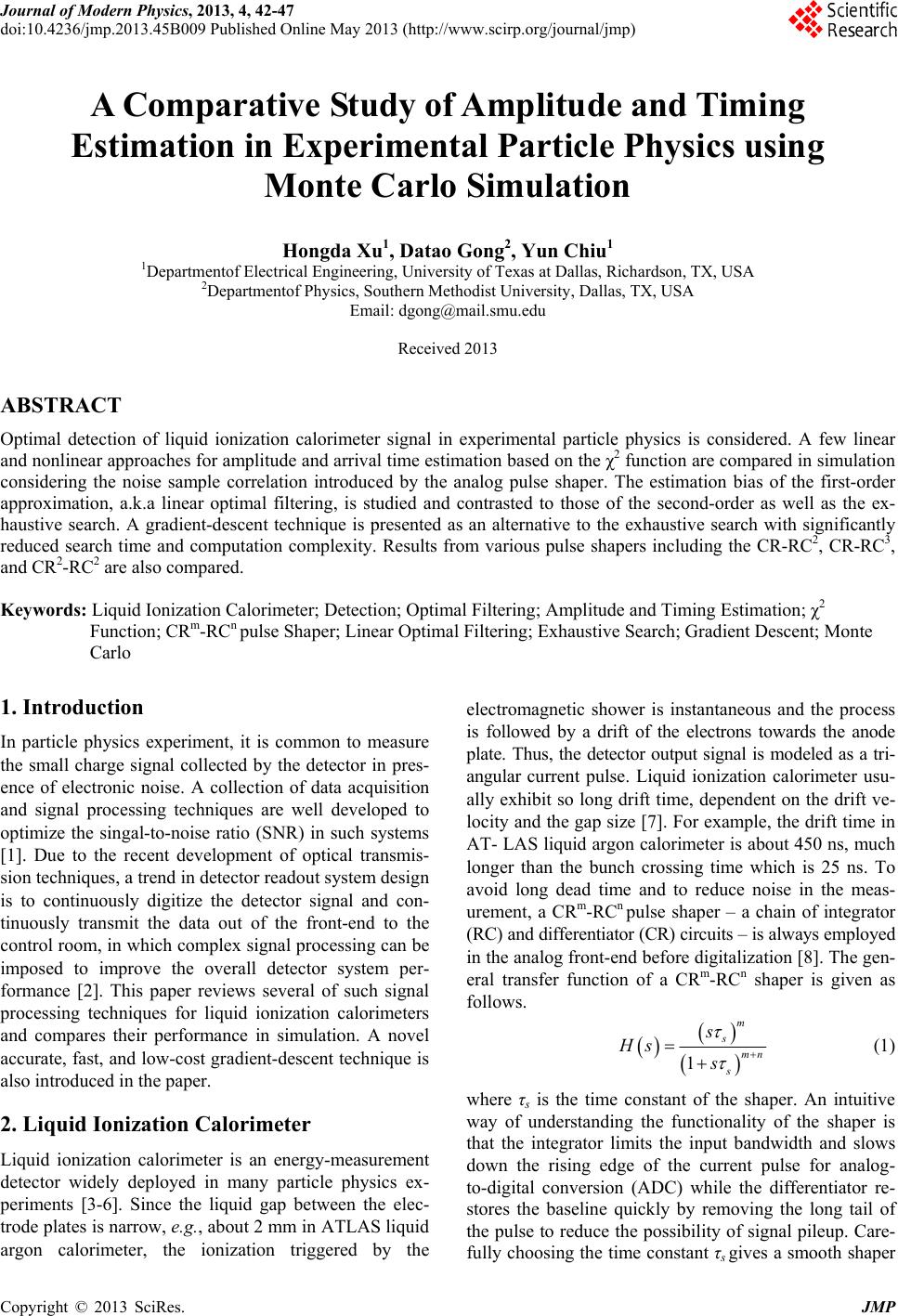
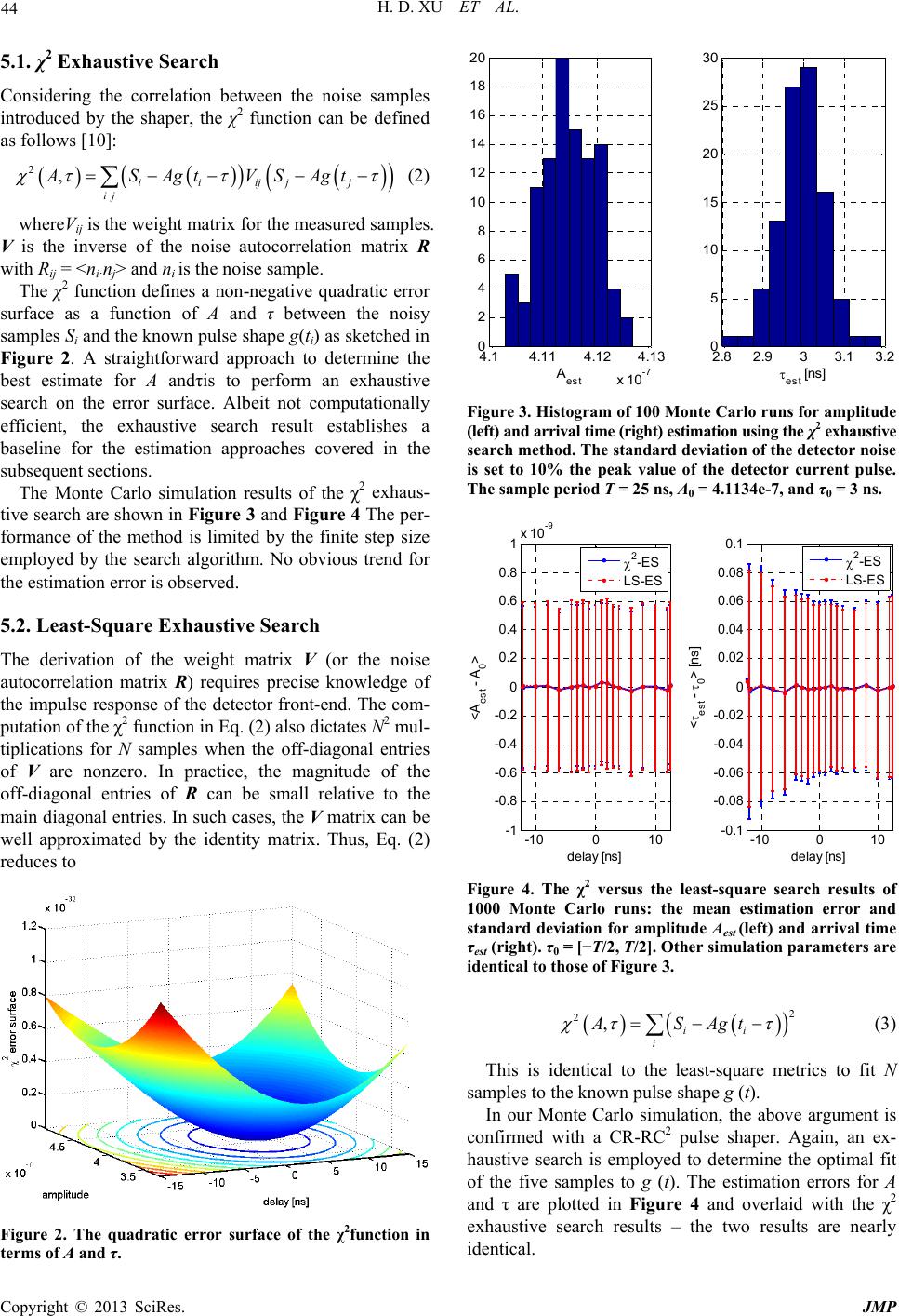
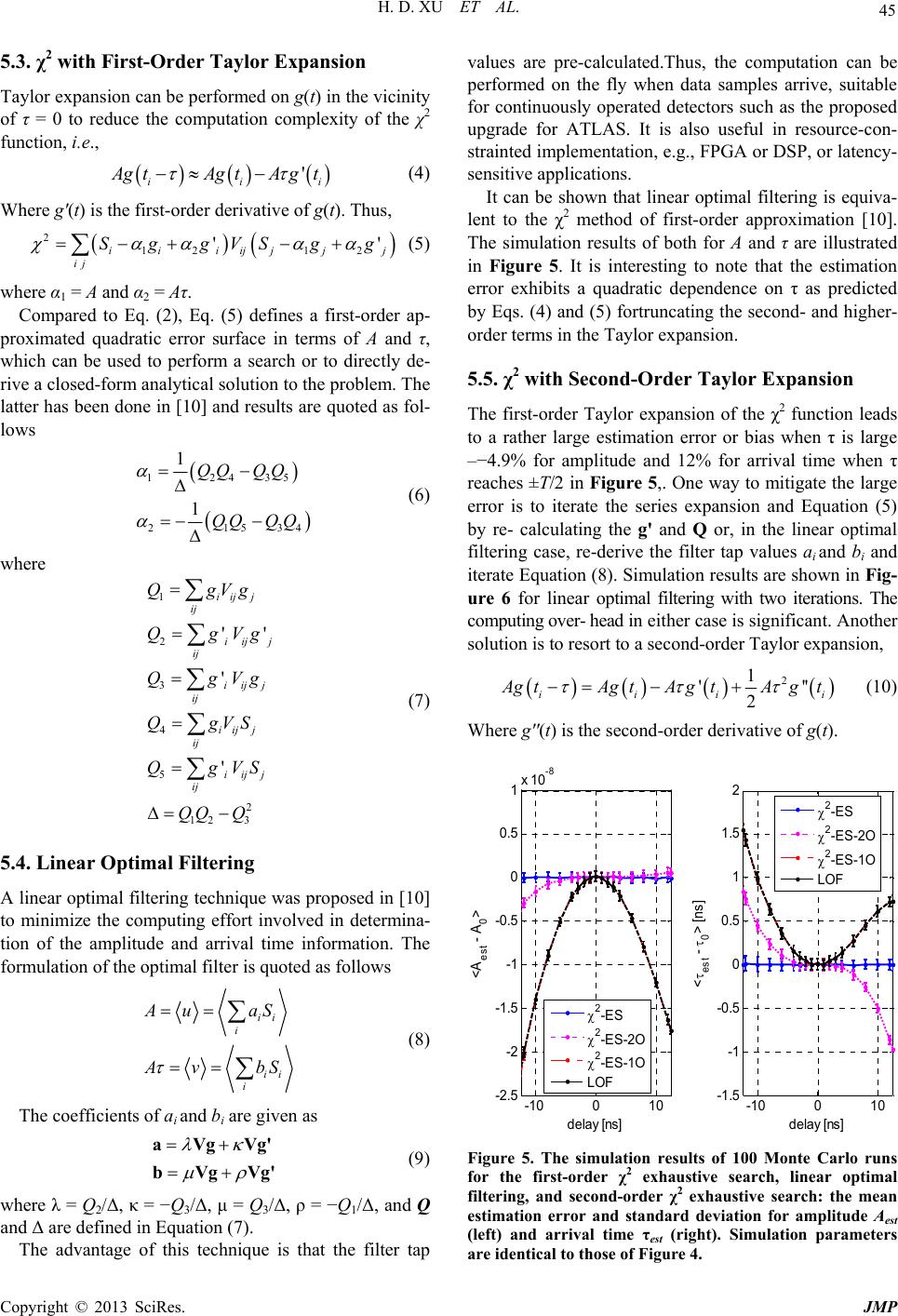
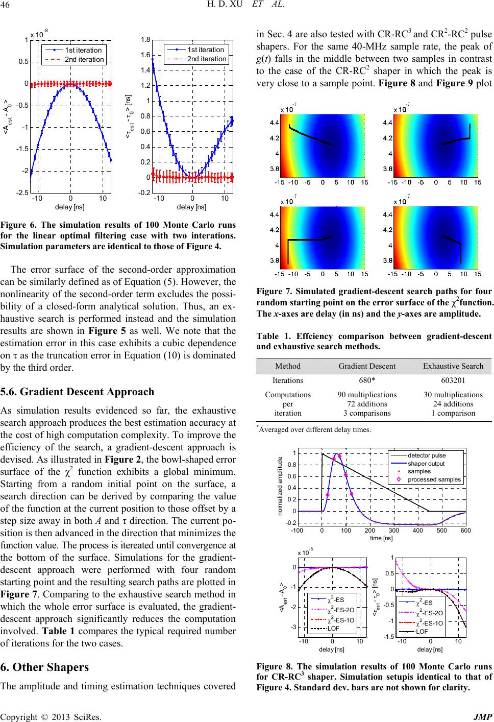
Copyright © 2013 SciRes. JMP