World Journal of Mechanics, 2013, 3, 215-223
doi:10.4236/wjm.2013.34021 Published Online July 2013 (http://www.scirp.org/journal/wjm)
Turbulent Flowfield Analysis in a Bluff-Body Burner
Using PIV
Nattan Roberto Caetano, Flávio Tadeu van der Laan
Department of Mechanical Engineering, University Federal of Rio Grande do Sul, Porto Alegre, Brazil
Received November 29, 2012; revised January 15, 2013; accepted January 23, 2013
Copyright © 2013 Nattan Roberto Caetano, Flávio Tadeu van der Laan. This is an open access article distributed under the Creative
Commons Attribution License, which permits unrestricted use, distribution, and reproduction in any medium, provided the original
work is properly cited.
ABSTRACT
The structure of inert turbulent flows, stabilized in a Bluff-Body burner, is studied considering different volumetric
flows for Nitrogen jet and annular air in coflow configuration. Flowfield analysis on Bluff-Body burner is essential to
improve the knowledge about this burner, which plays an important role in industrial applications. Thus, vector velocity
field is performed, employing Particle Image Velocimetry technique. Also, an uncertainty analysis is performed consid-
ering parameters involved in this technique yielding 6% to velocity measurements. The acquired information produces
the results based in flowfield structure, which are presented in terms of statistical momentum and Reynolds stress, in
which Boussinesq Hypothesis is considered to incompressible flows. However, this hypothesis fails in certain condi-
tions. In this way, is possible to comprehend and provide experimental data from the turbulent effects on the flowfield
and also contribute to predict the combustion flows, in order to enable the validation and develop numerical models.
Keywords: Particle Image Velocimetry; Turbulent Flowfield; Experimental Uncertainty; Boussinesq Hypothesis
1. Introduction
The aim of the work is study, experimentally, turbulent
flowfields stabilized on the Bluff-Body burner. Therefore,
measurements are performed using non-intrusive optical
technique in order to yield the velocity field, employing
PIV. This work intends to produce results which will
allow apply advanced post-processing methods. So that,
main experimental results are presented in order to verify
the flowfield structures characteristics, based in Boussi-
nesq Hypothesis. The knowledge yielded constitutes a
data base which enable developing and validation of nu-
merical models.
The present work emphasis is given by using the tech-
nique which allows measure the turbulent flowfield pro-
perties. Moreover, relevant aspects are approached, data
and statistical results processing. Velocity measurements
are necessary to investigate the turbulent flowfield struc-
ture and flow stabilization. However, this work focus on
the analysis of the flowfield dynamic influence on the
turbulence using velocity measures via Particle Image
Velocimetry PIV [1,2]. Measurements of vector velocity
field allow to perform the flowfield characterization by
the analysis of the results from statistical momentum, as
well as, through the flowfield Reynolds stresses tensor.
The flowfield stability depends on the interactions be-
tween dynamic, mixture and, chemical of the fluids con-
sidered. In this way, the velocity field structure plays an
important role on the numerical models development.
However, is a determinant factor in works which intend
to characterize the different flowfield structures. Thus,
both the diagnostic method purposed, followed by an
image post-processing, enriched the range of statistical
information available, such as a contribution toward the
information database creation, which allows comparisons
and numerical models calibration [3].
About parameters of the measure technique applied in
turbulent flowfield based on lasers, a trend is observed.
The capture rate used to measure reaching about kHz, in
one plane [4]. These measures covered small interroga-
tions areas, about some mm2, due the lasers energy limi-
tations. The size of the measurement window is smaller
than the normal techniques are able to capture, circa 100
cm2. Nowadays, the works perform 3D vector field ve-
locity, which is measured simultaneously with one scalar,
more often, OH or CH, or temperature [5,6]. High speed
equipment is employed in order to investigate turbulent
effects using information taken in high temporal resolu-
tion, in one or more planes [7]. Therefore, the results are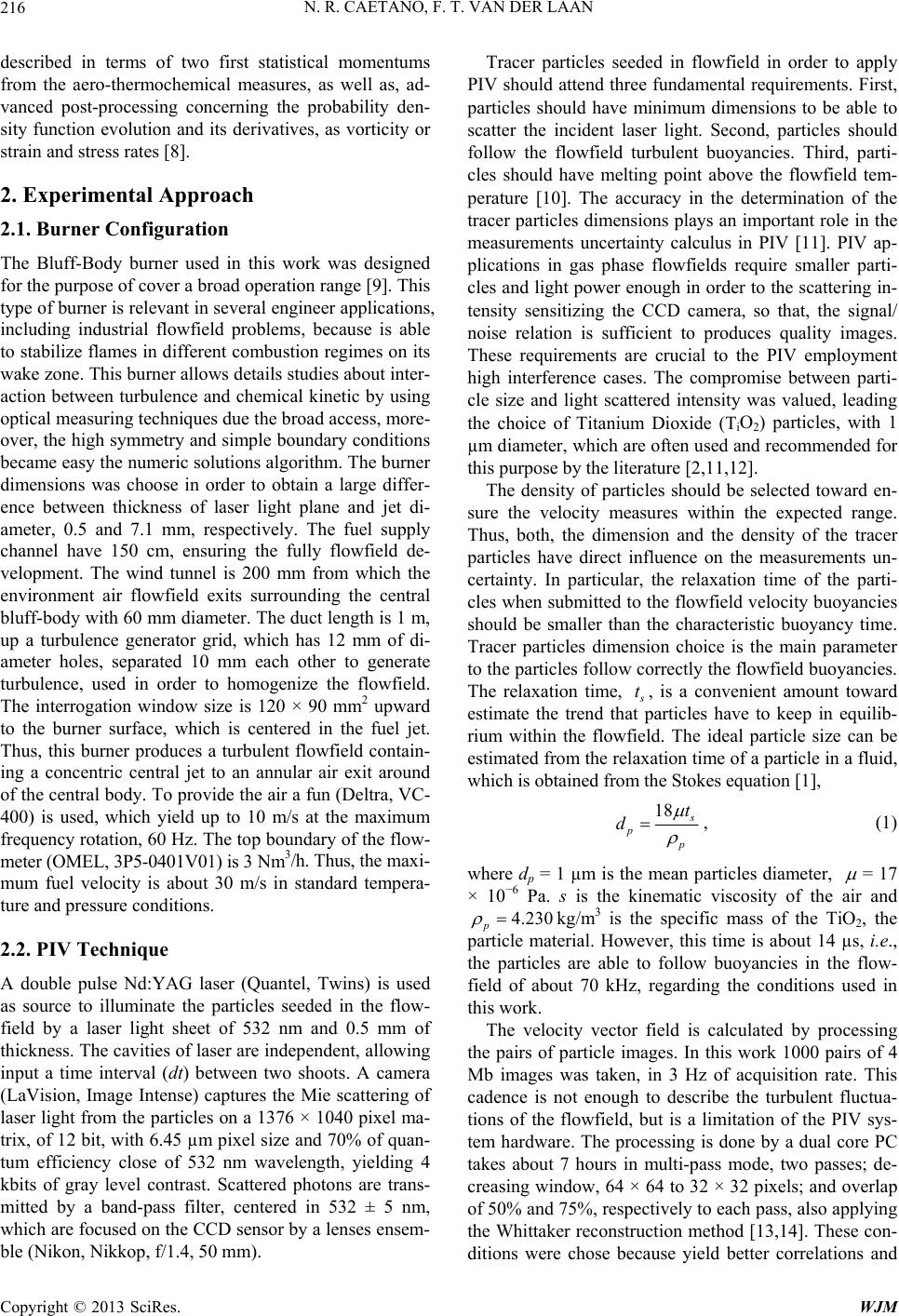

N. R. CAETANO, F. T. VAN DER LAAN 216
described in terms of two first statistical momentums
from the aero-thermochemical measures, as well as, ad-
vanced post-processing concerning the probability den-
sity function evolution and its derivatives, as vorticity or
strain and stress rates [8].
2. Experimental Approach
2.1. Burner Configuration
The Bluff-Body burner used in this work was designed
for the purpose of cover a broad operation range [9]. This
type of burner is relevant in several engineer applications,
including industrial flowfield problems, because is able
to stabilize flames in different combustion regimes on its
wake zone. This burner allows details studies about inter-
action between turbulence and chemical kinetic by using
optical measuring techniques due the broad access, more-
over, the high symmetry and simple boundary conditions
became easy the numeric solutions algorithm. The burner
dimensions was choose in order to obtain a large differ-
ence between thickness of laser light plane and jet di-
ameter, 0.5 and 7.1 mm, respectively. The fuel supply
channel have 150 cm, ensuring the fully flowfield de-
velopment. The wind tunnel is 200 mm from which the
environment air flowfield exits surrounding the central
bluff-body with 60 mm diameter. The duct length is 1 m,
up a turbulence generator grid, which has 12 mm of di-
ameter holes, separated 10 mm each other to generate
turbulence, used in order to homogenize the flowfield.
The interrogation window size is 120 × 90 mm2 upward
to the burner surface, which is centered in the fuel jet.
Thus, this burner produces a turbulent flowfield contain-
ing a concentric central jet to an annular air exit around
of the central body. To provide the air a fun (Deltra, VC-
400) is used, which yield up to 10 m/s at the maximum
frequency rotation, 60 Hz. The top boundary of the flow-
meter (OMEL, 3P5-0401V01) is 3 Nm3/h. Thus, the maxi-
mum fuel velocity is about 30 m/s in standard tempera-
ture and pressure conditions.
2.2. PIV Technique
A double pulse Nd:YAG laser (Quantel, Twins) is used
as source to illuminate the particles seeded in the flow-
field by a laser light sheet of 532 nm and 0.5 mm of
thickness. The cavities of laser are independent, allowing
input a time interval (dt) between two shoots. A camera
(LaVision, Image Intense) captures the Mie scattering of
laser light from the particles on a 1376 × 1040 pixel ma-
trix, of 12 bit, with 6.45 µm pixel size and 70% of quan-
tum efficiency close of 532 nm wavelength, yielding 4
kbits of gray level contrast. Scattered photons are trans-
mitted by a band-pass filter, centered in 532 ± 5 nm,
which are focused on the CCD sensor by a lenses ensem-
ble (Nikon, Nikkop, f/1.4, 50 mm).
Tracer particles seeded in flowfield in order to apply
PIV should attend three fundamental requirements. First,
particles should have minimum dimensions to be able to
scatter the incident laser light. Second, particles should
follow the flowfield turbulent buoyancies. Third, parti-
cles should have melting point above the flowfield tem-
perature [10]. The accuracy in the determination of the
tracer particles dimensions plays an important role in the
measurements uncertainty calculus in PIV [11]. PIV ap-
plications in gas phase flowfields require smaller parti-
cles and light power enough in order to the scattering in-
tensity sensitizing the CCD camera, so that, the signal/
noise relation is sufficient to produces quality images.
These requirements are crucial to the PIV employment
high interference cases. The compromise between parti-
cle size and light scattered intensity was valued, leading
the choice of Titanium Dioxide (TiO2) particles, with 1
µm diameter, which are often used and recommended for
this purpose by the literature [2,11,12].
The density of particles should be selected toward en-
sure the velocity measures within the expected range.
Thus, both, the dimension and the density of the tracer
particles have direct influence on the measurements un-
certainty. In particular, the relaxation time of the parti-
cles when submitted to the flowfield velocity buoyancies
should be smaller than the characteristic buoyancy time.
Tracer particles dimension choice is the main parameter
to the particles follow correctly the flowfield buoyancies.
The relaxation time,
s
t, is a convenient amount toward
estimate the trend that particles have to keep in equilib-
rium within the flowfield. The ideal particle size can be
estimated from the relaxation time of a particle in a fluid,
which is obtained from the Stokes equation [1],
18
s
p
p
t
d


, (1)
where dp = 1 µm is the mean particles diameter,

= 17
× 10−6 Pa. s is the kinematic viscosity of the air and
4.230
p


kg/m3 is the specific mass of the TiO2, the
particle material. However, this time is about 14 µs, i.e.,
the particles are able to follow buoyancies in the flow-
field of about 70 kHz, regarding the conditions used in
this work.
The velocity vector field is calculated by processing
the pairs of particle images. In this work 1000 pairs of 4
Mb images was taken, in 3 Hz of acquisition rate. This
cadence is not enough to describe the turbulent fluctua-
tions of the flowfield, but is a limitation of the PIV sys-
tem hardware. The processing is done by a dual core PC
takes about 7 hours in multi-pass mode, two passes; de-
creasing window, 64 × 64 to 32 × 32 pixels; and overlap
of 50% and 75%, respectively to each pass, also applying
the Whittaker reconstruction method [13,14]. These con-
ditions were chose because yield better correlations and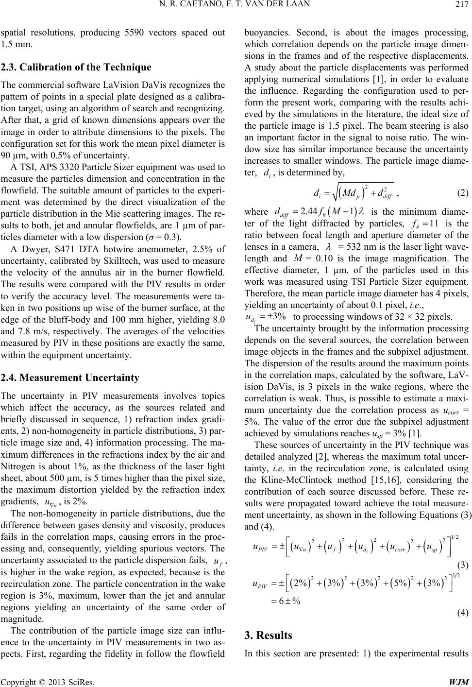

N. R. CAETANO, F. T. VAN DER LAAN 217
spatial resolutions, producing 5590 vectors spaced out
1.5 mm.
2.3. Calibration of the Technique
The commercial software LaVision DaVis recognizes the
pattern of points in a special plate designed as a calibra-
tion target, using an algorithm of search and recognizing.
After that, a grid of known dimensions appears over the
image in order to attribute dimensions to the pixels. The
configuration set for this work the mean pixel diameter is
90 µm, with 0.5% of uncertainty.
A TSI, APS 3320 Particle Sizer equipment was used to
measure the particles dimension and concentration in the
flowfield. The suitable amount of particles to the experi-
ment was determined by the direct visualization of the
particle distribution in the Mie scattering images. The re-
sults to both, jet and annular flowfields, are 1 µm of par-
ticles diameter with a low dispersion (σ = 0.3).
A Dwyer, S471 DTA hotwire anemometer, 2.5% of
uncertainty, calibrated by Skilltech, was used to measure
the velocity of the annulus air in the burner flowfield.
The results were compared with the PIV results in order
to verify the accuracy level. The measurements were ta-
ken in two positions up wise of the burner surface, at the
edge of the bluff-body and 100 mm higher, yielding 8.0
and 7.8 m/s, respectively. The averages of the velocities
measured by PIV in these positions are exactly the same,
within the equipment uncertainty.
2.4. Measurement Uncertainty
The uncertainty in PIV measurements involves topics
which affect the accuracy, as the sources related and
briefly discussed in sequence, 1) refraction index gradi-
ents, 2) non-homogeneity in particle distributions, 3) par-
ticle image size and, 4) information processing. The ma-
ximum differences in the refractions index by the air and
Nitrogen is about 1%, as the thickness of the laser light
sheet, about 500 µm, is 5 times higher than the pixel size,
the maximum distortion yielded by the refraction index
gradients, , is 2%.
n
The non-homogeneity in particle distributions, due the
difference between gases density and viscosity, produces
fails in the correlation maps, causing errors in the proc-
essing and, consequently, yielding spurious vectors. The
uncertainty associated to the particle dispersion fails,
u
f
u,
is higher in the wake region, as expected, because is the
recirculation zone. The particle concentration in the wake
region is 3%, maximum, lower than the jet and annular
regions yielding an uncertainty of the same order of
magnitude.
The contribution of the particle image size can influ-
ence to the uncertainty in PIV measurements in two as-
pects. First, regarding the fidelity in follow the flowfield
buoyancies. Second, is about the images processing,
which correlation depends on the particle image dimen-
sions in the frames and of the respective displacements.
A study about the particle displacements was performed
applying numerical simulations [1], in order to evaluate
the influence. Regarding the configuration used to per-
form the present work, comparing with the results achi-
eved by the simulations in the literature, the ideal size of
the particle image is 1.5 pixel. The beam steering is also
an important factor in the signal to noise ratio. The win-
dow size has similar importance because the uncertainty
increases to smaller windows. The particle image diame-
ter, , is determined by,
i
d

22
ip diff
dMdd, (2)
where


#
2.44 1
diff
dfM


is the minimum diame-
ter of the light diffracted by particles, # is the
ratio between focal length and aperture diameter of the
lenses in a camera,
11f

= 532 nm is the laser light wave-
length and
M
= 0.10 is the image magnification. The
effective diameter, 1 µm, of the particles used in this
work was measured using TSI Particle Sizer equipment.
Therefore, the mean particle image diameter has 4 pixels,
yielding an uncertainty of about 0.1 pixel, i.e.,
3%
i
d
u

 to processing windows of 32 × 32 pixels.
The uncertainty brought by the information processing
depends on the several sources, the correlation between
image objects in the frames and the subpixel adjustment.
The dispersion of the results around the maximum points
in the correlation maps, calculated by the software, LaV-
ision DaVis, is 3 pixels in the wake regions, where the
correlation is weak. Thus, is possible to estimate a maxi-
mum uncertainty due the correlation process as ucorr =
5%. The value of the error due the subpixel adjustment
achieved by simulations reaches usp = 3% [1].
These sources of uncertainty in the PIV technique was
detailed analyzed [2], whereas the maximum total uncer-
tainty, i.e. in the recirculation zone, is calculated using
the Kline-McClintock method [15,16], considering the
contribution of each source discussed before. These re-
sults were propagated toward achieve the total measure-
ment uncertainty, as shown in the following Equations (3)
and (4).

 


1/2
2 22
22
i
PIVnfdcorr sp
uuuuuu



 




(3)

12
22222
2% 3% 3% 5% 3%
6%
PIV
u


 



(4)
3. Results
In this section are presented: 1) the experimental results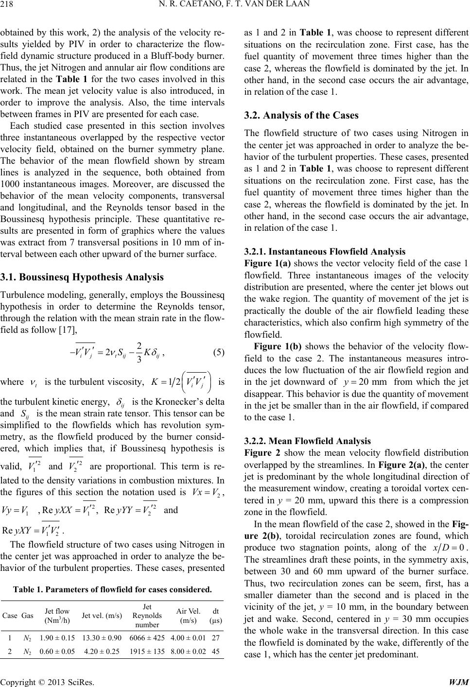

N. R. CAETANO, F. T. VAN DER LAAN 218
obtained by this work, 2) the analysis of the velocity re-
sults yielded by PIV in order to characterize the flow-
field dynamic structure produced in a Bluff-body burner.
Thus, the jet Nitrogen and annular air flow conditions are
related in the Table 1 for the two cases involved in this
work. The mean jet velocity value is also introduced, in
order to improve the analysis. Also, the time intervals
between frames in PIV are presented for each case.
Each studied case presented in this section involves
three instantaneous overlapped by the respective vector
velocity field, obtained on the burner symmetry plane.
The behavior of the mean flowfield shown by stream
lines is analyzed in the sequence, both obtained from
1000 instantaneous images. Moreover, are discussed the
behavior of the mean velocity components, transversal
and longitudinal, and the Reynolds tensor based in the
Boussinesq hypothesis principle. These quantitative re-
sults are presented in form of graphics where the values
was extract from 7 transversal positions in 10 mm of in-
terval between each other upward of the burner surface.
3.1. Boussinesq Hypothesis Analysis
Turbulence modeling, generally, employs the Boussinesq
hypothesis in order to determine the Reynolds tensor,
through the relation with the mean strain rate in the flow-
field as follow [17],
2
23
ij tijij
VVS K



 , (5)
where t

is the turbulent viscosity, 12 ij
K
VV






is
the turbulent kinetic energy, ij

is the Kronecker’s delta
and ij is the mean strain rate tensor. This tensor can be
simplified to the flowfields which has revolution sym-
metry, as the flowfield produced by the burner consid-
ered, which implies that, if Boussinesq hypothesis is
S
valid,
2
1
V and 2
2
V are proportional. This term is re-
lated to the density variations in combustion mixtures. In
the figures of this section the notation used is 2
Vx V

,
1
Vy V ,22
12
Re, ReyXXVyYY V

 and
12
Re yXYV V

.
The flowfield structure of two cases using Nitrogen in
the center jet was approached in order to analyze the be-
havior of the turbulent properties. These cases, presented
Table 1. Parameters of flowfield for cases considered.
Case Gas Jet flow
(Nm3/h) Jet vel. (m/s)
Jet
Reynolds
number
Air Vel.
(m/s)
dt
(µs)
1 N2 1.90 ± 0.15 13.30 ± 0.906066 ± 425 4.00 ± 0.0127
2 N2 0.60 ± 0.05 4.20 ± 0.251915 ± 135 8.00 ± 0.0245
as 1 and 2 in Table 1, was choose to represent different
situations on the recirculation zone. First case, has the
fuel quantity of movement three times higher than the
case 2, whereas the flowfield is dominated by the jet. In
other hand, in the second case occurs the air advantage,
in relation of the case 1.
3.2. Analysis of the Cases
The flowfield structure of two cases using Nitrogen in
the center jet was approached in order to analyze the be-
havior of the turbulent properties. These cases, presented
as 1 and 2 in Table 1, was choose to represent different
situations on the recirculation zone. First case, has the
fuel quantity of movement three times higher than the
case 2, whereas the flowfield is dominated by the jet. In
other hand, in the second case occurs the air advantage,
in relation of the case 1.
3.2.1. Instantaneous Flowfield Analysis
Figure 1(a) shows the vector velocity field of the case 1
flowfield. Three instantaneous images of the velocity
distribution are presented, where the center jet blows out
the wake region. The quantity of movement of the jet is
practically the double of the air flowfield leading these
characteristics, which also confirm high symmetry of the
flowfield.
Figure 1(b) shows the behavior of the velocity flow-
field to the case 2. The instantaneous measures intro-
duces the low fluctuation of the air flowfield region and
in the jet downward of 20 mmy

from which the jet
disappear. This behavior is due the quantity of movement
in the jet be smaller than in the air flowfield, if compared
to the case 1.
3.2.2. Mean Flowfield Analysis
Figure 2 show the mean velocity flowfield distribution
overlapped by the streamlines. In Figure 2(a), the center
jet is predominant by the whole longitudinal direction of
the measurement window, creating a toroidal vortex cen-
tered in y = 20 mm, upward this there is a compression
zone in the flowfield.
In the mean flowfield of the case 2, showed in the Fig-
ure 2(b), toroidal recirculation zones are found, which
produce two stagnation points, along of the 0xD

.
The streamlines draft these points, in the symmetry axis,
between 30 and 60 mm upward of the burner surface.
Thus, two recirculation zones can be seem, first, has a
smaller diameter than the second and is placed in the
vicinity of the jet, y = 10 mm, in the boundary between
jet and wake. Second, centered in y = 30 mm occupies
the whole wake in the transversal direction. In this case
the flowfield is dominated by the wake, differently of the
case 1, which has the center jet predominant.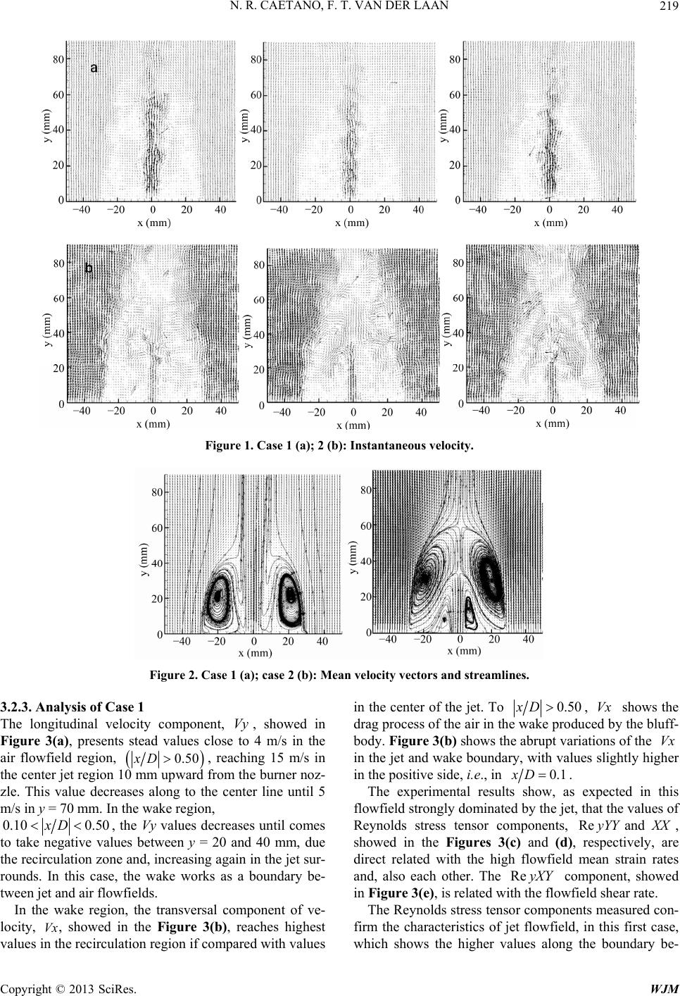

N. R. CAETANO, F. T. VAN DER LAAN 219
Figure 1. Case 1 (a); 2 (b): Instantaneous velocity.
Figure 2. Case 1 (a); case 2 (b): Mean velocity vectors and streamlines.
3.2.3. Analysis of Case 1
The longitudinal velocity component, Vy , showed in
Figure 3(a), presents stead values close to 4 m/s in the
air flowfield region,

0.50xD, reaching 15 m/s in
the center jet region 10 mm upward from the burner noz-
zle. This value decreases along to the center line until 5
m/s in y = 70 mm. In the wake region,
0.10 0.50xD
, the Vy values decreases until comes
to take negative values between y = 20 and 40 mm, due
the recirculation zone and, increasing again in the jet sur-
rounds. In this case, the wake works as a boundary be-
tween jet and air flowfields.
In the wake region, the transversal component of ve-
locity, , showed in the Figure 3(b), reaches highest
values in the recirculation region if compared with values
in the center of the jet. To
Vx
0.50xD, shows the
drag process of the air in the wake produced by the bluff-
body. Figure 3(b) shows the abrupt variations of the
in the jet and wake boundary, with values slightly higher
in the positive side, i.e., in
Vx
Vx
0.1xD.
The experimental results show, as expected in this
flowfield strongly dominated by the jet, that the values of
Reynolds stress tensor components, ,
showed in the Figures 3(c) and (d), respectively, are
direct related with the high flowfield mean strain rates
and, also each other. The component, showed
in Figure 3(e), is related with the flowfield shear rate.
Re and yYY XX
Re yXY
The Reynolds stress tensor components measured con-
firm the characteristics of jet flowfield, in this first case,
which shows the higher values along the boundary be-

N. R. CAETANO, F. T. VAN DER LAAN 220
Figure 3. Case 1: Evolution in transversal direction (x), to longitudinal positions spaced 10 mm from the burner surface, of
the components longitudinal (Vy) and transversal (Vx) of the velocity [m/s] and the components ReyXX, YY and XY [m2/s2]. ―
10, - - 20, • • 30, - • - 40, – – 50, - • • 60, • • • 70 mm.
tween jet and wake, where the highest strain rates are
found. The components, , are small in the
air flowfield region, circa 0.1 m2/s2, where the velocity
gradient is zero, see Figure 3(a). In this same region
is null, indicating that there is turbulence isot-
ropy. The stress values increases to 0.5 m2/s2 in the wake
region, mainly upward to the recirculation zone, 40 < y <
70 mm. The maximum values occurs in the jet/wake
boundary, where ReyXX = 2, ReyYY = 7 and ReyXY = 2
m2/s2. Note that, in the central side of the jet the values of
Reynolds stress components decreases close the burner
surface, i.e., to y < 20 mm.
Re ,yXX YY
Re yXY
An analysis of the ReyXY and ReyXX results showed
in the Figures 3(c) and (d), allows verifying that the
Boussinesq hypothesis is satisfied, due two reasons. First,
both stress values corresponds to the higher mean strain
rate, second, there is a direct relation between ReyXY and
. The Figure 3(e) analysis also allows verifying
that there is a proportionality between the mean strain
rate for shear and . Thus, within the experimen-
tal uncertainty of the results, the Boussinesq hypothesis
to incompressible flowfields is satisfied in the whole
Re yXX
Re yXY

N. R. CAETANO, F. T. VAN DER LAAN 221
region. In the wake, 0.10 0.50xD , seems occurs a
low deviation to the normal stress proportionality, nev-
ertheless, this is due the difficulty in measure accurately
the small values of if compared with values.
Vx Vy
3.2.4. Analysis of Case 2
The values of keep steady close to 8 m/s in the air
flowfield region,
Vy
0.50xD. Along the center line this
velocity component reaches 7 m/s in the maximum at 10
mm upward to the burner surface, decreasing drastically
to −2 m/s within 40 < y < 60 mm. Upward to y = 70 mm
the mixture region becomes homogeneous and tends to
be dominated by the air flowfield, which has Vy = 1 m/s.
Figure 4(a) shows the evolution of the values from the
measurements results performed in the case 2 to several
heights above the burner surface. The velocity compo-
nent, , allows to note that upward to y = 30 mm there
is a strong interaction between jet and air along the
whole wake region, producing intense turbulence, evi-
dent in the Reynolds stress profiles. The jet is broken in y
Vy
Figure 4. Case 2: Evolution in transversal direction (x), to longitudinal positions spaced 10 mm from the burner surface, of
the components longitudinal (Vy) and transversal (Vx) of the velocity [m/s] and the components ReyXX, YY and XY [m2/s2]. ―
10, - - - 20, • • • 30, - • - 40, – – – 50, - • • 60, • • • 70 mm.

N. R. CAETANO, F. T. VAN DER LAAN 222
= 40 mm, where a jet and air mixture is intense, consis-
tent with the jet scattering process occurred in the wake
region. In the wake region, the transversal component of
velocity, , showed in the Figure 4(b), reaches high-
est values in the recirculation region near the wake and
air boundary. Figure 4(b) shows the minor variations of
the in the jet and wake boundary.
Vx
Vx
The Reynolds stress tensor components, Figures 4(c)-
(e), confirm that, in the case 2, the flowfield characteris-
tics are dominated by the wake. The component
shows the local maximum values, 2 m2/s2, in
Re yXY
x
D
and
0.500.10xD. These values increase gradu-
ally until y = 40 mm, in particular, reaches values close
to those achieved in case 1, whose jet is predominant,
circa 2 m2/s2. The comparison of Figures 4(c) and (d)
suggests that ReyXX and ReyYY are not proportional, i.e.,
the Boussinesq hypothesis should not be used as model
in order to simulate this flowfield.
The component ReyXX is practically uniform in the
wake region, where the highest measured values evolutes
from downward to upward, which intensify and spread in
the region that air and wake mixture occurs.
The component ReyXY presents a maximum absolute
value of in 1 m2/s2 wake region. From downward to up-
ward ReyXY is transported from the air and wake bound-
ary, 0.50xD, in direction to the center, 0xD

.
This is other indicative that the flowfield structure is
dominated by the wake.
The Boussinesq hypothesis is not sufficient to descrip-
tion of the turbulent transport of the case 2 flowfield,
instead of the case 1. However, a mathematic model de-
signed to numerical simulation of this flowfield should
use a Reynolds stress transport model.
4. Conclusions
The detailed characterization of the turbulent flowfield
requires, necessarily, the velocity distribution with a spa-
tial resolution such as allows to analyze the interaction of
the vortex in the large scale and the turbulence isotropy.
The detailed velocity field distribution allows the devel-
opment of the new models, which are able to describe the
different combustion regimes.
Future works intend to employ the stereo PIV tech-
nique, which allows a reconstruction of the measure-
ments toward obtain 3D results, in order to produce more
information, i.e., the nine components of the Reynolds
tensor. Thus, will be possible the calculation of those
three anisotropy components [17].
In this work were presented results of the turbulent
flowfield characterization from a nitrogen jet and annular
air in coflow configuration, stabilized upward a bluff-
body burner. These results are important regarding the
representation of the industrial conditions and prepare to
analyze reaction conditions. The main advantages of the
optical technique used in this work, PIV, are the non-
intrusive measurements, the high resolution images re-
sults and the low uncertainty. The achieved results allow
to visualization of the flowfield detailed structure, de-
signed for the vector velocity field. Furthermore, the tho-
rough measurements uncertainty analysis yielded 6%.
The instantaneous images allow to note that as the
flowfield turbulence quantity increases the variations of
the intern structure grows up. These local characteristics
hamper the numerical simulations of the flowfield. The
data results about the velocity distribution provide infor-
mation to development and validation of the new com-
putational models in order to improve combustion sys-
tems projects and numerical simulations.
REFERENCES
[1] M. Raffel, C. E. Willert, S. T. Wereley and J. Kompen-
hans, “Particle Image Velocimetry, a Praticle Guide,”
Göttingen, Springer, 2007, p. 448.
[2] J. Westerweel, “Fundamentals of Digital Particle Image
Velocimetry,” Measurement Science and Technology,
Vol. 8, No. 12, 1997, pp. 1379-1392.
doi:10.1088/0957-0233/8/12/002
[3] N. R. Caetano, “Estudo Experimental de Chamas Tur-
bulentas não Pré-Misturadas Empregando Simultanea-
mente as Técnicas de Diagnóstico Laser PLIF e PIV,”
Ph.D. Thesis, Mechanical Engineering Department, PUC-
Rio, Rio de Janeiro, 2012, p. 180.
[4] B. Böhm, C. Heeger, I. Boxx, W. Meier and A. Dreizler,
“Time-Resolved Conditional Flow Field Statistics in Ex-
tinguishing Turbulent Opposed Jet Flames Using Simul-
taneous High Speed PIV/OH-PLIF,” Proceedings of the
Combustion Institute, Vol. 32, No. 2, 2009, pp. 1647-
1654. doi:10.1016/j.proci.2008.06.136
[5] P. S. Kothnur, M. S. Tsurikov, N. T. Clemens, J. M. Don-
bar and C. D. Carter, “Planar Imaging of CH, OH, and
Velocity in Turbulent Non-Premixed Jet Flames,” Pro-
ceedings of the Combustion Institute, Vol. 29, No. 2,
2002, pp. 1921-1927.
doi:10.1016/S1540-7489(02)80233-4
[6] A. M. Steinberg, J. F. Driscoll and S. L. Ceccio, “Tem-
poral Evolution of Flame Stretch Due to Turbulence and
the Hydrodynamic Instability,” Proceedings of the Com-
bustion Institute, Vol. 32, No. 2, 2009, pp. 1713-1721.
doi:10.1016/j.proci.2008.05.003
[7] M. Shimura, T. Ueda, G. Choi, M. Tanahashi and T. Mi-
yauchi, “Simultaneous Dual-Plane CH PLIF, Single-
Plane OH PLIF and Dual-Plane Stereoscopic PIV Meas-
urements in Methane-Air Turbulent Premixed Flames,”
Proceedings of the Combustion Institute, Vol. 33, No. 1,
2011, pp. 775-782. doi:10.1016/j.proci.2010.05.026
[8] G. Troiani, M. Marrocco, S. Giammartini and C. M. Cas-
ciola, “Counter-Gradient Transport in the Combustion of
a Premixed CH4/Air Annular Jet by Combined PIV/
OH-LIF,” Combustion and Flame, Vol. 156, No. 3, 2009,
pp. 608-620. doi:10.1016/j.combustflame.2008.12.010

N. R. CAETANO, F. T. VAN DER LAAN 223
[9] L. E. A. Huapaya, “Caracterização Numérica e Experi-
mental de Uma Chama Turbulenta não Pré-Misturada,”
Ph.D. Thesis, Mechanical Engineering Department, PUC-
Rio, Rio de Janeiro, 2008, p. 169.
[10] P. T. Lacava and C. A. Martins, “Métodos Experimentais
de Análise Aplicados à Combustão,” Papel Brasil, 2010.
[11] A. P. S. Freire, A. Ilha and R. Breidenthal, “Turbulência,”
5th Turbulence and Transition School, IME, Rio de Ja-
neiro, 2006.
[12] P. Petersson, J. Olofsson, C. Brackman, H. Seyfried, J.
Zetterberg, M. Richter, M. Aldén, M. A. Linne, R. K.
Cheng, A. Nauert, D. Geyer and A. Dreizler, “Simulta-
neous PIV/OH-PLIF, Rayleigh Thermometry/OH-PLIF
and Stereo PIV Measurements in a Low-Swirl Flame,”
Applied Optics, Vol. 46, No. 9, 2007, pp. 3928-3936.
doi:10.1364/AO.46.003928
[13] E. T. Whittaker, “Expansions of the Interpolation-Theory,”
Proceedings of the Royal Society, Vol. 35, 1915, p. 181.
[14] T. Roesgen, “Optimal Subpixel Interpolation in Particle
Image Velocimetry,” Experiments in Fluids, Vol. 35, No.
3, 2003, pp. 252-256. doi:10.1007/s00348-003-0627-8
[15] S. J. Kline and F. A. McClintock, “Describing Uncertain-
ties in Single-Sample Experiments,” Mechanical Engi-
neering, 1953.
[16] R. J. Moffat, “Contributions to the Theory of Single-Sam-
ple Uncertainty Analysis,” Journal of Fluids Engineering,
Vol. 104, No. 2, 1982, pp. 250-258.
doi:10.1115/1.3241818
[17] S. B. Pope, “Turbulent Flows,” Cambridge, 2000, p. 749.
doi:10.1017/CBO9780511840531
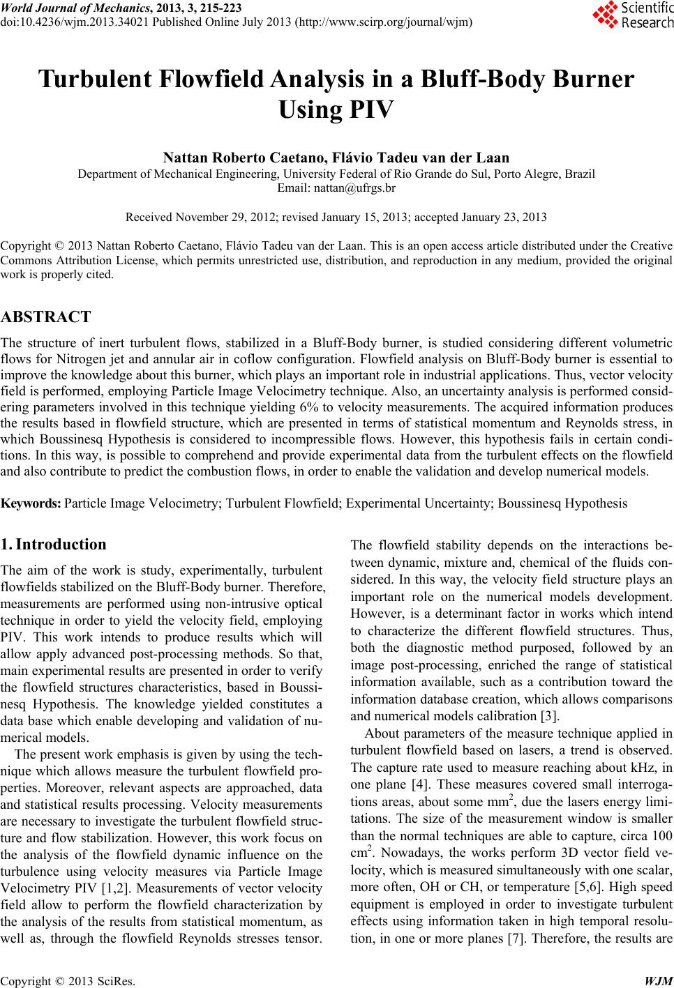