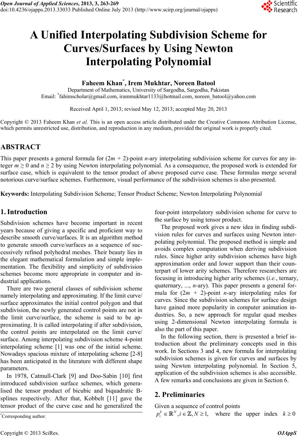
 Open Journal of Applied Sciences, 2013, 3, 263-269 doi:10.4236/ojapps.2013.33033 Published Online July 2013 (http://www.scirp.org/journal/ojapps) A Unified Interpolating Subdivision Scheme for Curves/Surfaces by Using Newton Interpolating Polynomial Faheem Khan*, Irem Mukhtar, Noreen Batool Department of Mathematics, University of Sargodha, Sargodha, Pakistan Email: *fahimscholar@gmail.com, irammukhtar1133@hotmail.com, noreen_batool@yahoo.com Received April 1, 2013; revised May 12, 2013; accepted May 20, 2013 Copyright © 2013 Faheem Khan et al. This is an open access article distributed under the Creative Commons Attribution License, which permits unrestricted use, distribution, and reproduction in any medium, provided the original work is properly cited. ABSTRACT This paper presents a general formula for (2m + 2)-point n-ary interpolating subdivision scheme for curves for any in- teger m ≥ 0 and n ≥ 2 by using Newton interpolating polynomial. As a consequence, the proposed work is extended for surface case, which is equivalent to the tensor product of above proposed curve case. These formulas merge several notorious curve/surface schemes. Furthermore, visual performance of the subdivision schemes is also presented. Keywords: Interpolating Subdivision Scheme; Tensor Product Scheme; Newton Interpolating Polynomial 1. Introduction Subdivision schemes have become important in recent years because of giving a specific and proficient way to describe smooth curve/surfaces. It is an algorithm method to generate smooth curve/surfaces as a sequence of suc- cessively refined polyhedral meshes. Their beauty lies in the elegant mathematical formulation and simple imple- mentation. The flexibility and simplicity of subdivision schemes become more appropriate in computer and in- dustrial applications. There are two general classes of subdivision scheme namely interpolating and approximating. If the limit curve/ surface approximates the initial control polygon and that subdivision, the newly generated control points are not in the limit curve/surface, the scheme is said to be ap- proximating. It is called interpolating if after subdivision, the control points are interpolated on the limit curve/ surface. Among interpolating subdivision scheme 4-point interpolating scheme [1] was one of the initial scheme. Nowadays spacious mixture of interpolating scheme [2-8] has been anticipated in the literature with different shape parameters. In 1978, Catmull-Clark [9] and Doo-Sabin [10] first introduced subdivision surface schemes, which genera- lised the tensor product of bicubic and biquadratic B- splines respectively. After that, Kobbelt [11] gave the tensor product of the curve case and he generalized the four-point interpolatory subdivision scheme for curve to the surface by using tensor product. The proposed work gives a new idea in finding subdi- vision rules for curves and surfaces using Newton inter- polating polynomial. The proposed method is simple and avoids complex computation when deriving subdivision rules. Since higher arity subdivision schemes have high approximation order and lower support than their coun- terpart of lower arity schemes. Therefore researchers are focusing in introducing higher arity schemes (i.e., ternary, quaternary, ..., n-ary). This paper presents a general for- mula for (2m + 2)-point n-ary interpolating rules for curves. Since the subdivision schemes for surface design have gained more popularity in computer animation in- dustries. So, a new approach for regular quad meshes using 2-dimensional Newton interpolating formula is also the part of this paper. In the following section, there is presented a brief in- troduction about the preliminary concepts used in this work. In Sections 3 and 4, new formula for interpolating subdivision schemes is given for curves and surfaces by using Newton interpolating polynomial. In Section 5, application of the subdivision schemes is also accessible. A few remarks and conclusions are given in Section 6. 2. Preliminaries Given a sequence of control points ,,1 kN i piN, where the upper index 0k *Corresponding author. Copyright © 2013 SciRes. OJAppS  F. KHAN ET AL. 264 indicates the subdivision level. An n-ary subdivision curve is defined by 1 , 0 ,0,1,..., 1, m kk niji j j pap n n (2.1) where m > 0 and , 0 1,0,1,..., 1. m j j a (2.2) The set of coefficients ,j 0 ,0,1,...,1 m an is called subdivision mask. In the limit the proc- ess (2.1) defines an infinite set of points in The sequence of control points ,k . N k i p 1 is connected, in a natural way, with the diadic mesh points The process then defines a scheme whereby and replaces the values and at the mesh points S and 1ni n i /, kk i tini 1k ni p 1 k i p1k ni p . 1k ni n p k i p k tk t respectively, while is inserted at the new mesh points 1 1 1() kk nii i tnt n k t for 1,2,...,1.n Labeling of old and new points is shown in Figure 1, which illustrates subdivision scheme (2.1). Let 21mbe the space of all polynomials of degree where m is non-negative integer. If 1, 1m 2m j m x is fundamental Newton polynomial corre- sponding to the node point 1m m j 1 is defined by 21 m mj jm Px aNx j (2.3) In general, the coefficient of the Newton form of polynomial is called divided difference, the divided dif- ference 0n is a symmetric function, hence can be found by following method, [x,..., x], j ay , , [,..., ], , mmj ji mj m j im imik yxx p apx xxx ik j (2.4) and can originate by the subsequent way, Ν(x) j 1 1, ,, j j km kj Nx ikkj (2.5) 3. Construction of the Subdivision Scheme for Univariate Case This section gives the construction of (2m + 2)-point bi- nary and ternary interpolating schemes. Then by induc- tion, a general formula for (2m + 2)-point n-ary interpo- lating subdivision scheme is formulated for curve case. 3.1. (2m + 2)-Point Binary Interpolating Scheme To construct the rules for binary 2-point interpolating scheme, consider 1 0 j x be the Fundamental Newton polynomial to the node points {0, 1}. The New- ton polynomial replicate linear polynomial P in the way that taking m = 0 in (2.3), we achieve 1 1 0 , jj j PxaN x (3.1) where j is divided difference can be calculated by (2.4), and by setting in (2.5). This implies that a Ν(x) j 1010 1 00 11 x Pxpp px Cp C , (3.2) with following Gamma function 1. 11 xx Cx Now, to construct the desired 2-point ternary subdivi- sion scheme, let 11 21 211 1 0, . 2 ii ppip pi Since we want to construct uniform and stationary scheme reproducing polynomials up to a fixed degree, it is sufficient to consider the case i = 0 with subdivision level k = 0. This implies that (a) (b) (c) Figure 1. Solid lines show coarse polygons whereas dotted lines are refined polygons. (a)-(c) represent binary, ternary and quaternary refinement of coarse polygon using (2.1) for n = 2, 3, 4 respectively. Copyright © 2013 SciRes. OJAppS  F. KHAN ET AL. 265 10 (0) ,pp 10 11 1 . 22 2 pp 1 p Now as an affine combination of 2-point 11 1 ,, kk ii pp we suppose that at (k + 1)th level, the point 1 2 ki p is attached to the parametric value 1 2, 2k i so the desired binary 2-point interpolating subdivision scheme is given by 1 2 1 21 1 , 11 . 22 kk ii kk ii pp ppp k i 0,1 (3.3) In composite form (3.3) can be written as 1 1 2 00 11 , kx ii pCpC (3.4) where 1,. 11 kx i x pC x x 2 Continuing in the same way for m = 1 in (2.3), where be the Newton polynomial to the node points {−1, 0, 1, 2} then we have the following compact form of 4-point binary subdivision scheme Ν(x) j 1 2 31 1 00 11 , ki x i p Cp C 0,1 (3.5) where 12,. 21 xx Cx x 2 Consequently, we can generate a general form of (2m + 2)-point binary interpolating scheme, which is of the following form 21 1 2 00 11 m kx ii im pCp ,C m (3.6) where 1,0, 11 xm xm Cxm 1 corresponding to , 2 xm 0 and subdivision level 0.k 3.2. (2m + 2)-Point Ternary Interpolating Scheme To construct the rules for ternary 4-point interpolating scheme, consider 2 1 jj x be the Newton polyno- mial to the node points {−1, 0, 1, 2}. The Newton poly- nomial reproduces cubic polynomial P in the way that taking m = 1 in (2.3), we achieve 2 3 1 . jj j PxaN x (3.7) Now by using (2.4) and (2.5) in (3.5), we have 3101 2 101 3 2101 31 1 00 1 12 2 133 6 11 x i Pxpp px pppxx ppppxx Cp C . (3.8) Now to construct the 4-point ternary subdivision scheme, take 11 1 33 313323 12 0, ,. 33 ii i ppip pippi (3.9) From (3.7) and (3.8), we get 30 0,pp 3101 3101 1520 104 2 2 , 381 272780 2410205 , 381272780 ppp ppp p p we attain the following iterative rules for ternary 4-point interpolating subdivision scheme, 1 3 1 3111 2 1 3211 2 , 520104 , 8127 2780 410205 . 8127 2780 kk ii kkkk iiii kkkk iiii pp pppp pppp k i k i p p 1,2 (3.10) In composite form, the above rules can be written as 3 11 31 00 11 ,0, kkx ii pCpC (3.11) where 2,. 21 xx Cx x 3 Accordingly, general formula for (2m + 2)-point ter- nary interpolating scheme is given by 21 1 3 00 11 m kx iim pCp , m C (3.12) Copyright © 2013 SciRes. OJAppS  F. KHAN ET AL. 266 where 1,0,1, 11 xm xm Cxm 2 corresponding to , 3 xm 0 ,C and subdivision level 0.k 3.3. (2m + 2)-Point n-Ary Interpolating Subdivision Sc h e me (Ge n er a l ization) Now there is presented a general formula for (2m + 2)- point n-ary (i.e. binary, ternary and so on) interpolating subdivision scheme by using Newton interpolating poly- nomial. This new formula will be helpful to drive inter- polating subdivision rule plainly and quickly. The gen- eral formula for (2m + 2)-point n-ary interpolating subdi- vision scheme has the following form 21 1 00 11 m kx ni im pCp m (3.13) where 1,0,1,..., 1 11 xm xm Cn xm corresponding to ,xm n 0 and indicates 0k the subdivision level, where n stand for n-ary scheme. Remark 3.1. In the following, we see that some other well-known interpolating schemes come from our pro- posed Formula (3.13). Setting the value of m = 1, and n = 2, in above result, which is the 4-point DD scheme [12], 1 2 1 2111 2 , 1991 . 1616 1616 kk ii kkkk iiii pp pppp k i p By setting m = 2, and n = 2, in proposed result, we get 6-point DD scheme [12], 1 2 1 212 1 12 , 32575 256256 128 75253 . 128 256256 kk ii kkkk iiii kk ii pp pppp pp 3 k i p Taking m = 1, and n = 3 in (3.13), we get ternary 4-point interpolating scheme [13], 1 2 1 3111 2 1 3211 2 , 520204 , 8127 2781 420205 8127 2781 kk ii kkkk iiii kkkk iiii pp pppp pppp By setting m = 2, and n = 3 in (3.13), we get ternary 6-point interpolating scheme [13], 1 2 1 3111 2 1 3211 2 , 520204 , 81272781 420205 81272781 kk ii kkkk iiii kkkk iiii pp pppp pppp k i k i p p 2, 4. Tensor Product of (2m + 2)-Point n-Ary Interpolating Subdivision Scheme Given a sequence of control points , , kN ij p ,,ij N where the upper index indicates the subdivision level. An n-ary subdivision surface scheme in the tensor product form is defined by 0k 1 ,,,, 00 , ,0,1,...,1, mm kk ninjrsir js rs paap n (4.1) where ,0 m rr a and ,s 0 m s a satisfy (2.2). Given ini- tial values 0 ,,, , N ij pij p then in the limit the process (4.1) defines an infinite set of points in The sequence of values is related, in a natu- k . N , k ij ral way, with the diadic mesh points ,,, kk ijij nn . The process then defines a scheme whereby 1 , k ni nj p replaces the value at the mesh point /,/ k injn p // , kk injn nn for ,(0,n), while the val- ues 1 , k ni nj p are inserted at the new mesh points 1 , k nj nn 1k ni for ,0,1,...,n1. Labeling of old and new points is shown in Figure 2 which illustrates subdivision scheme (4.1). Here, we present a general formula for tensor product of (2m+2)-point n-ary interpolating scheme in the fol- lowing form, 12 12 12 12 12 12 12 212 1 1 , 00 00 11 mm k ninj p 121122 121 2 112 2 ,, xm xm imj m CC pCC (4.2) where 11 1 22 2 11 111 1 22 222 2 1, 11 1. 11 xm xm xm Cxm xm Cxm k i k i p p Copyright © 2013 SciRes. OJAppS 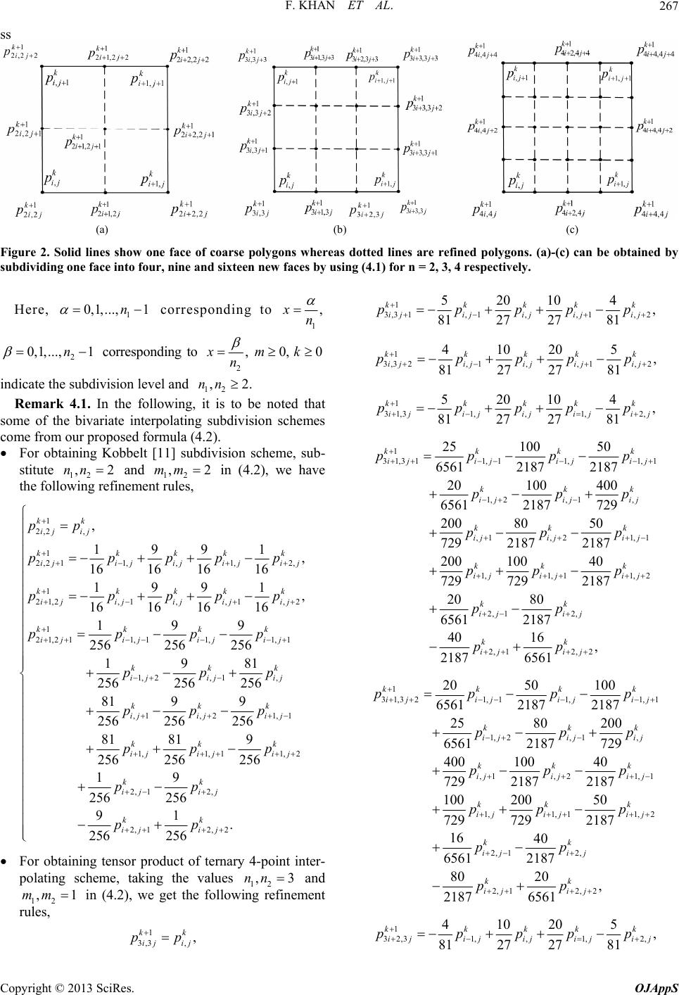 F. KHAN ET AL. Copyright © 2013 SciRes. OJAppS 267 ss (a) (b) (c) Figure 2. Solid lines show one face of coarse polygons whereas dotted lines are refined polygons. (a)-(c) can be obtained by subdividing one face into four, nine and sixteen new faces by using (4.1) for n = 2, 3, 4 respectively. Here, 1 3,3 1, 1,, 1,2 52010 4 , 8127 2781 kkkk i jijijijij pppp 1 0,1,..., 1n corresponding to 1 n,x k p 2 0,1,..., 1n corresponding to 2 ,xn 0, 0mk 1 3,32, 1, 410205 , 81 27 kkkkk i jijij ppppp , 1,2 27 81 ij ij indicate the subdivision level and . k 4.1. In the foat somhe bivariate interpes come from our pr). For obtainingivision scheme, sub in (4.2), we have 12 ,2nn Remar llowing, it is to be noted th e of tolating subdivision schem 1 31,31, ,1,2, 520104 , 8127 2781 kkkkk ijij ij ijij ppppp oposed formula (4.2 Kobbelt [11] subd- 1k p 3 1,311,11,1,1 1,2, 1, ,1 ,21,1 1,1, 11,2 25100 50 65612187 2187 20100400 65612187729 200 8050 729 21872187 200 10040 729 7292187 20 6561 kkk ijijij ij kkk i jijij kk k ijiji j kk k ij ijij ppp ppp ppp pp p stitute 12 ,2nn and 12 ,2mm the following refinement rules, 1 2,2, , kk ij ij pp 1 2, 2 11,,1,2, 1 1991 , 16 1616 16 199 kk kkk ijij ij ij ij kkk pp ppp ppp 21 ,2, 1,,1,2 1 21,2 11,11,1, 1 1, 2 1 , 16 1616 16 199 256256 256 19 256 256 kk i jijijijij kkkk i jijijij k ij i pp pppp pp ,1, ,1 ,21,1 1,1, 11,2 2, 12, 2, 12,2 81 256 81 99 256 256256 81 819 256 256256 19 256 256 91 . 256 256 kk jij kk k ijiji j kk k ijijij kk ij ij kk ij ij p ppp pp p pp pp For obtaining tensor product of ternary 4-point inter- polating scheme, taking the values 2, 12, 2, 12,2 80 2187 4016 , 2187 6561 kk ijij kk ij ij pp pp 1 3 1,321,11,1,1 1,2,1, ,1 ,21,1 1,1, 11,2 2050100 65612187 2187 2580 200 65612187 729 400 10040 729 21872187 100 20050 729 7292187 16 6561 kkk i jijijij kk i jijij kk k ijiji j kk k ij ijij ppp pp ppp pp p k k p p 2, 12, 2, 12, 2 40 2187 8020 , 2187 6561 kk ij ij kk ijij pp pp 12 ,3nn and in (4.2), we get the folloent 12 ,1mm rules, wing refinem 1 32,31,,1,2, 410205 , 8127 2781 kkkk ijijijiji j pppp k p 1 3,3,, kk ij ij pp 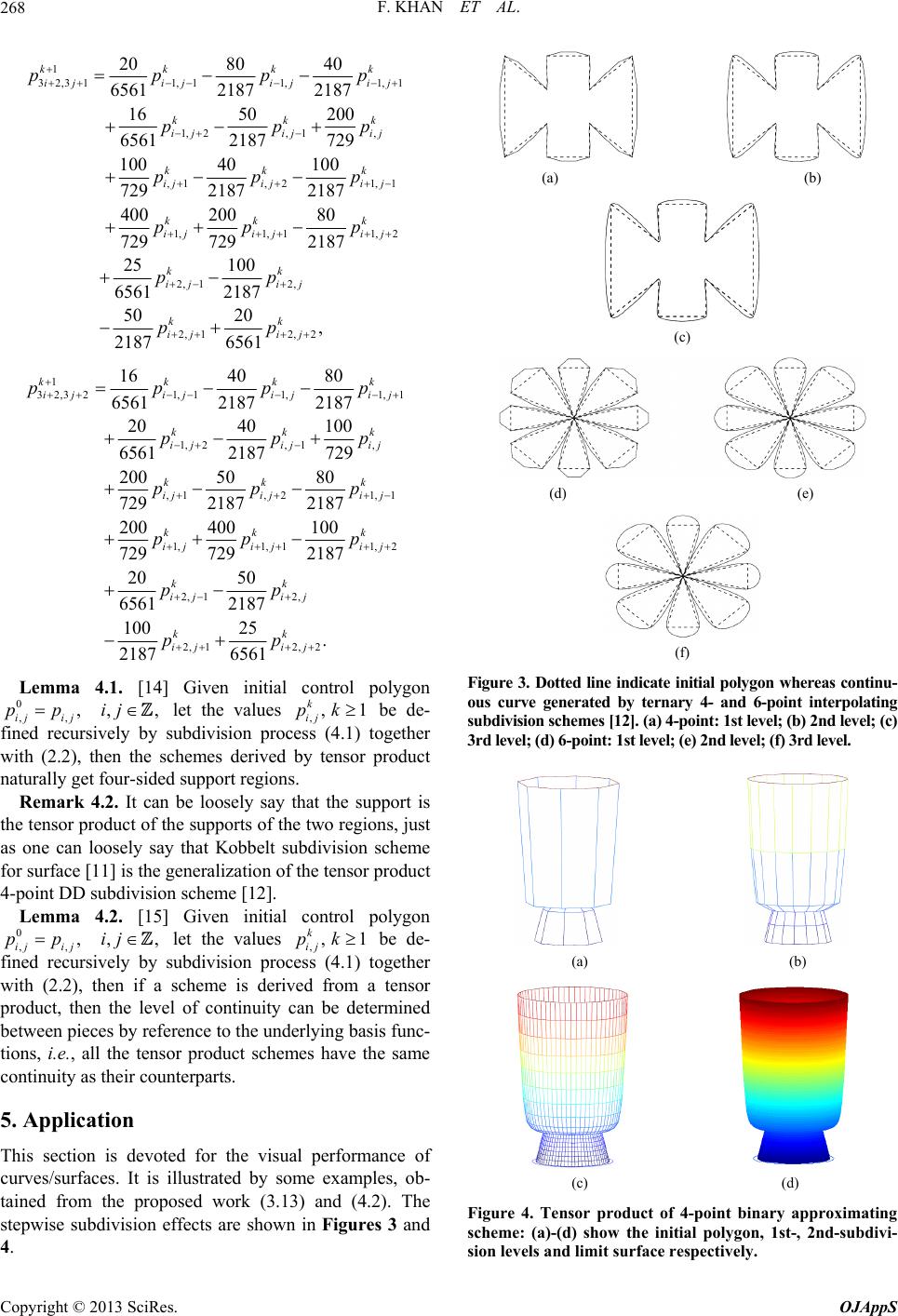 F. KHAN ET AL. 268 1 3 2,311,11,1,1 1,2,1, ,1 ,21,1 1,1, 11,2 2080 40 65612187 2187 1650 200 65612187 729 100 40100 729 21872187 400 20080 729 7292187 25 6561 kkk i jijijij kk ijijij kk k ijiji j kk k ij ijij ppp pp ppp pp p p k k p p 2, 12, 2, 12,2 100 2187 5020 , 2187 6561 kk ijij kk ij ij p pp 1 3 2,321,11,1,1 1,2, 1, ,1 ,21,1 1,1, 11,2 1640 80 65612187 2187 2040100 65612187 729 200 5080 729 21872187 200 400100 729 7292187 20 6561 kkk i jijijij kk i jijij kk k ijiji j kk k ijijij ppp pp ppp pp p p k k p p 2, 12, 2, 12,2 50 2187 10025 . 2187 6561 kk ij ij kk ijij p pp Lemma 4.1. [14] Given initial control polygon let the values be de- subdivision pgether with (2.2), then the schemes derived by tensor product naturally get four-sided support regions. Remark 4.2. It can be loosely say that the support is the tensor product of the supports of the two regions, just as one can loosely say that Kobbelt subdivision scheme for surface [11] is the generalization of the tensor prodct 4-point DD subdivision scheme [12]. Lemma 4.2. [15] Given initial control polygon let the values be de- subdivision pgether with (2.2), then if a scheme is derived from a tensor product, then the level of continuity can be determined between pieces by reference to the underlying basis func- tio continuity as their cou 0 ,, , ij ij pp fined recu ,,ij rsively by ,,1 k ij pk rocess (4.1) to u 0 ,, , ij ij pp fined recu ,,ij rsively by ,,1 k ij pk rocess (4.1) to ns, i.e., all the tensor product schemes have the same nterparts. 5. Application This section is devoted for the visual performance of curves/surfaces. It is illustrated by some examples, ob- tained from the proposed work (3.13) and (4.2). The stepwise subdivision effects are shown in Figures 3 and 4. (a) (b) (c) (d) (e) (f) Figure 3. Dotted line indicate initial polygon whereas continu- ous curve generated by terna- and 6-point interpolating subdivision schemes [12]. (a) 4t: 1st level; (b) 2nd level; (c) 3rd level; (d) 6-point: 1st level; (e) 2nd level; (f) 3rd level. ry 4 -poin (a) (b) (c) (d) Figure 4. Tensor product of 4-point binary approximating scheme: (a)-(d) show the initial polygon, 1st-, 2nd-subdivi- sion levels and limit surface respectively. Copyright © 2013 SciRes. OJAppS 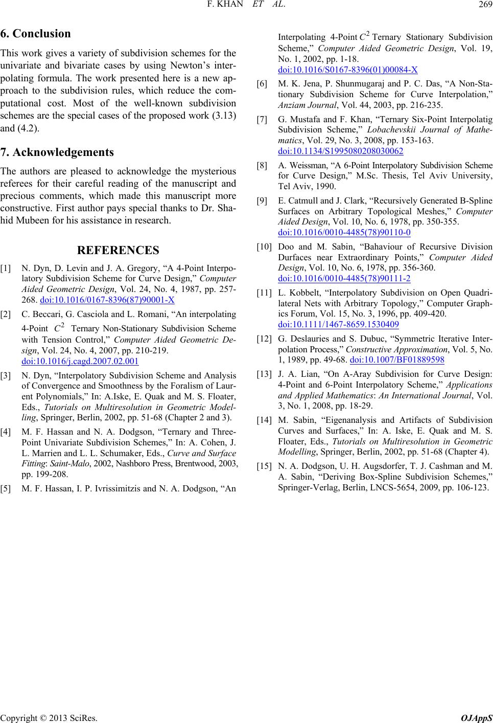 F. KHAN ET AL. Copyright © 2013 SciRes. OJAppS 269 6. Conclusion This work gives a variety of subdivision schemes for the univariate and bivariate cases by using Newton’s inter- polating formula. The work presented here is a new ap- proach to the subdivision rules, which reduce the com putational cost. Most of the well-known subdivision schemes are the special cases of the proposed work (3.13) and (4.2). 7. Acknowledgements The authors are pleased to acknowledge the mysterious referees for their careful reading of the manuscript and precious comments, which made this manuscript more constructive. First author pays special thanks to Dr. Sha- hid Mubeen for his assistance in research. Interpolating 4-Point2 CTernary Stationary Subdivision Scheme,” Computer Aided Geometric Design, Vol. 19, No. 1, 2002, pp. 1-18. doi:10.1016/S0167-8396(01)00084-X [6] M. K. Jena, P. Shunmugaraj and P. C. Das, “A Non-Sta- tionary Subdivision Scheme for Curve Interpolation,” Anziam Journal, Vol. 44, 2003, pp. 216-235. [7] G. Mustafa and F. Khan, “Ternary Six-Point Interpolatig Subdivision Scheme,” Lobachevskii Journal of Mathe- - matics, Vol. 29, No. 3, 2008, pp. 153-163. doi:10.1134/S1995080208030062 [8] A. Weissman, “A 6-Point Interpolatory Subdivision Scheme for Curve Design,” M.Sc. Thesis, Tel Aviv University, Tel Aviv, 1990. [9] E. Catmull and J. Clark, “Recursively Generated B-Spline Surfaces on Arbitrary Topological Meshes,” Computer Aided Design, Vol. 10, No. 6, 1978, pp. 350-355. doi:10.1016/0010-4485(78)90110-0 [10] Doo and M. Sabin, “Bahaviour of Recursive Division Durfaces near Extraordinary Points,” Computer Aided Design, Vol. 10, No. 6, 1978, pp. 356-360. doi:10.1016/0010-4485(78)90111-2 REFERENCES [1] N. Dyn, D. Levin and J. A. Gregory, “A 4-Point Interpo- latory Subdivision Scheme for Curve Design,” Computer Aided Geometric Design, Vol. 24, No. 4, 1987, pp. 257- 268. doi:10.1016/0167-8396(87)90001-X pp. 409-420. [11] L. Kobbelt, “Interpolatory Subdivision on Open Quadri- lateral Nets with Arbitrary Topology,” Computer Graph- ics Forum, Vol. 15, No. 3, 1996, asciola and L. Romani, “An interpolating[2] C. Beccari, G. C doi:10.1111/1467-8659.1530409 [12] G. Deslauries and S. Dubuc, “Symmetric Iterative Inter- polation Process,” Constructive Approximation, Vol. 1, 1989, pp. 49-68. 4-Point 2 C Ternary Non-Stationary Subdivision Scheme with Tension Control,” Computer Aided Geometric De- sign, Vol. 24, No. 4, 2007, pp. 210-219. doi:10.1016/j.cagd.2007.02.001 [3] N. Dyn, “Interpolatory Subdivision Scheme and Analysis of Convergence and Smoothness by the Foralism of Laur- ent Polynomials,” In: A.Iske, E. Quak and M. S. Floater, Eds., T ling, Springer 5, No. 889598doi:10.1007/BF01 utorials on Multiresolution in Geometric Model- , Berlin, 2002, pp. 51-68 (Chapter 2 and 3) odgson, “Ternary and Three- Schemes,” In: A. Cohen, J. . [4] M. F. Hassan and N. A. D Point Univariate Subdivision L. Marrien and L. L. Schumaker, Eds., Curve and Surface Fitting: Saint-Malo, 2002, Nashboro Press, Brentwood, 2003, pp. 199-208. [5] M. F. Hassan, I. P. Ivrissimitzis and N. A. Dodgson, “An ournal, Vol. eometric . 51-68 (Chapter 4). . 106-123. [13] J. A. Lian, “On A-Aray Subdivision for Curve Design: 4-Point and 6-Point Interpolatory Scheme,” Applications and Applied Mathematics: An International J 3, No. 1, 2008, pp. 18-29. [14] M. Sabin, “Eigenanalysis and Artifacts of Subdivision Curves and Surfaces,” In: A. Iske, E. Quak and M. S. Floater, Eds., Tutorials on Multiresolution in G Modelling, Springer, Berlin, 2002, pp [15] N. A. Dodgson, U. H. Augsdorfer, T. J. Cashman and M. A. Sabin, “Deriving Box-Spline Subdivision Schemes,” Springer-Verlag, Berlin, LNCS-5654, 2009, pp
|