 Journal of Modern Physics, 2013, 4, 26-41 http://dx.doi.org/10.4236/jmp.2013.47A1004 Published Online July 2013 (http://www.scirp.org/journal/jmp) Application of the Non-Local Physics in the Theory of Gravitational Waves and Big Bang Boris V. Alexeev Physics Department, Moscow Lomonosov State University of Fine Chemical Technologies, Moscow, Russia Email: Boris.Vlad.Alexeev@gmail.com Received April 7, 2013; revised May 10, 2013; accepted June 15, 2013 Copyright © 2013 Boris V. Alexeev. This is an open access article distributed under the Creative Commons Attribution License, which permits unrestricted use, distribution, and reproduction in any medium, provided the original work is properly cited. ABSTRACT The theory of gravitational waves in the frame of non-local quantum hydrodynamics (NLQH) is considered. From cal- culations follow that NLQH equations for “empty” space have the traveling wave solutions belonging in particular to the soliton class. The possible influence and reaction of the background microwave radiation is taken into account. These results lead to the principal correction of the inflation theory and serve as the explanation for the recent discovery of the universe’s cosmic microwave background anomalies. The simple analytical particular cases and numerical calcu- lations are delivered. Proposal for astronomers—to find in the center domain of the hefty cold spot the smallest hot spot as the origin of the initial burst—Big Bang. Keywords: Foundations of the Theory of Transport Processes; The Theory of Solitons; Generalized Hydrodynamic Equations; Foundations of Quantum Mechanics; Traveling Wave Solutions; Big Bang 1. Introduction More than ten years ago, the accelerated cosmological expansion was discovered in direct astronomical obser- vations at distances of a few billion light years, almost at the edge of the observable Universe. This acceleration should be explained because mutual attraction of cosmic bodies is only capable of decelerating their scattering. It means that we reach the revolutionary situation not only in physics but also in the natural philosophy on the whole. As result, new idea was introduced in physics about ex- isting of a force with the opposite sign, which is called universal antigravitation. Its physical source is called as dark energy that manifests itself only because of postu- lated property of providing antigravitation. It was postulated that the source of antigravitation is “dark matter” which inferred to exist from gravitational effects on visible matter. However, from the other side dark matter is undetectable by emitted or scattered elec- tromagnetic radiation. It means that new essences—dark matter, dark energy—were introduced in physics only with the aim to account for discrepancies between meas- urements of the mass of galaxies, clusters of galaxies and the entire universe made through dynamical and general relativistic means, measurements based on the mass of the visible “luminous” matter. It could be reasonable if we are speaking about small corrections to the system of knowledge achieved by mankind to the time we are liv- ing. But mentioned above discrepancies lead to affirma- tion, that dark matter constitutes 80% of the matter in the universe, while ordinary matter makes up only 20%. Practically we are in front of the new challenge since Newton’s Mathematical Principles of Natural Philoso- phy was published. Dark matter was postulated by Swiss astrophysicist Fritz Zwicky [1,2] of the California Institute of Tech- nology in 1933. He applied the virial theorem to the Coma cluster of galaxies and obtained evidence of un- seen mass. Zwicky estimated the cluster’s total mass based on the motions of galaxies near its edge and com- pared that estimate to one based on the number of galax- ies and total brightness of the cluster. He found that there was about 400 times more estimated mass than was visu- ally observable. The gravity of the visible galaxies in the cluster would be far too small for such fast orbits, so something extra was required. This is known as the “missing mass problem”. Based on these conclusions, Zwicky inferred that there must be some non-visible form of matter, which would provide enough of the mass, and gravity to hold the cluster together. Observations have indicated the presence of dark mat- ter in the universe, including the rotational speeds of galaxies, gravitational lensing of background objects by C opyright © 2013 SciRes. JMP  B. V. ALEXEEV 27 galaxy clusters such as the Bullet Cluster, and the tem- perature distribution of hot gas in galaxies and clusters of galaxies. The work by Vera Rubin (see for example [3,4]) re- vealed distant galaxies rotating so fast that they should fly apart. Outer stars rotated at essentially the same rate as inner ones (~254 km/s). This is in marked contrast to the solar system where planets orbit the sun with veloci- ties that decrease as their distance from the centre in- creases. By the early 1970s, flat rotation curves were routinely detected. It was not until the late 1970s, however, that the community was convinced of the need for dark matter halos around spiral galaxies. The mathematical modeling (based on Newtonian mechanics and local phy- sics) of the rotation curves of spiral galaxies was realized for the various visible components of a galaxy (the bulge, thin disk, and thick disk). These models were unable to predict the flatness of the observed rotation curve beyond the stellar disk. The inescapable conclusion, assuming that Newton’s law of gravity (and the local physics de- scription) holds on cosmological scales, that the visible galaxy was embedded in a much larger dark matter (DM) halo, which contributes roughly 50% - 90% of the total mass of a galaxy. As result other models of gravitation were involved in consideration—from “improved” New- tonian laws (such as modified Newtonian dynamics and tensor-vector-scalar gravity [5]) to the Einstein’s theory based on the cosmological constant [6]. Einstein intro- duced this term as a mechanism to obtain a stable solu- tion of the gravitational field equation that would lead to a static universe. Computer simulations with taking into account the hypothetical DM in the local hydrodynamic description include usual moment equations plus Poisson equation with different approximations for the density of DM DM containing several free parameters. Computer si- mulations of cold dark matter (CDM) predict that CDM particles ought to coalesce to peak densities in galactic cores. However, the observational evidence of star dy- namics at inner galactic radii of many galaxies, including our own Milky Way, indicates that these galactic cores are entirely devoid of CDM. No valid mechanism has been demonstrated to account for how galactic cores are swept clean of CDM. This is known as the “cuspy halo problem”. As result, the restricted area of CDM influence introduced in the theory. As we can see that the concept of DM leads to many additional problems. I do not intend to review the different speculations based on the principles of local physics. I see another problem. It is the problem of Oversimplification—but not “trivial” simplification of the important problem. The situation is much more serious—total Oversimplification based on principles of local physics, and obvious crisis, we see in astrophysics, simply reflects the general short- enings of the local kinetic transport theory. In other words returning to the previous problems—is it possible using only Newtonian gravitation law and non-local statistical description to forecast the Hubble expansion and flat gravitational curve of a typical spiral galaxy? Both ques- tions have the positive answers [7]. Another extremely important class of cosmological problems is connected with gravitational waves, universe inflation and anomalies in the distribution of the uni- verse’s cosmic microwave background (CMB). This class of problems leads also to antigravitation but in absolutely another sense. In other words what is the origin of the Big Bang and evolution in the burst regime when “usual” matter and “dark” matter do not exist on principle? Let us investigate the possibilities which deliver the unified generalized quantum hydrodynamics [8-12] for investigation of these problems. I deliver here some main ideas and deductions of the generalized Boltzmann physi- cal kinetics and non-local physics. For simplicity, the fundamental methodic aspects are considered from the qualitative standpoint of view avoiding excessively cum- bersome formulas. A rigorous description can be found, for example, in the monographs [8-11], see also [12-17]. Let us consider the transport processes in open dissi- pative systems and ideas of following transformation of generalized hydrodynamic description in quantum hy- drodynamics which can be applied to the individual par- ticle. The kinetic description is inevitably related to the sys- tem diagnostics. Such an element of diagnostics in the case of theoretical description in physical kinetics is the concept of the physically infinitely small volume (PhSV). The correlation between theoretical description and sys- tem diagnostics is well-known in physics. Suffice it to recall the part played by test charge in electrostatics or by test circuit in the physics of magnetic phenomena. The traditional definition of PhSV contains the statement to the effect that the PhSV contains a sufficient number of particles for introducing a statistical description; however, at the same time, the PhSV is much smaller than the volume V of the physical system under consideration; in a first approximation, this leads to the local approach in investigating of the transport processes. It is assumed in classical hydrodynamics that local thermodynamic equi- librium is first established within the PhSV, and only after that the transition occurs to global thermodynamic equilibrium if it is at all possible for the system under study. Let us consider the hydrodynamic description in more detail from this point of view. Assume that we have two neighboring physically infinitely small volumes PhSV1 and PhSV2 in a non-equilibrium system. Even the point- like particles (starting after the last collision near the boundary between two mentioned volumes) can change Copyright © 2013 SciRes. JMP  B. V. ALEXEEV 28 the distribution functions in the neighboring volume. The adjusting of the particles dynamic characteristics for translational degrees of freedom takes several collisions in the simplest case. As result, we have in the definite sense “the Knudsen layer” between these volumes. This fact unavoidably leads to fluctuations in mass and hence in other hydrodynamic quantities. Existence of such “Knudsen layers” is not connected with the choice of space nets and fully defined by the reduced description for ensemble of particles of finite diameters in the con- ceptual frame of open physically small volumes, there- fore—with the chosen method of measurement. This en- tire complex of effects defines non-local effects in space and time. The physically infinitely small volume (PhSV) is an open thermodynamic system for any division of macro- scopic system by a set of PhSVs. But the Boltzmann equation (BE) [8,18,19] Df DtJ, (1.1) where is the Boltzmann collision integral and DDt is a substantive derivative, fully ignores non-local effects and contains only the local collision integral . The foregoing nonlocal effects are insignificant only in equi- librium systems, where the kinetic approach changes to methods of statistical mechanics. This is what the difficulties of classical Boltzmann physical kinetics arise from. Also a weak point of the classical Boltzmann kinetic theory is the treatment of the dynamic properties of interacting particles. On the one hand, as follows from the so-called “physical” derivation of BE, Boltzmann particles are regarded as material points; on the other hand, the collision integral in the BE leads to the emergence of collision cross sections. Notice that the application of the above principles also leads to the modification of the system of Maxwell equa- tions. While the traditional formulation of this system does not involve the continuity equation, its derivation explicitly employs the equation 0 a j r a a t , (1.2) where is the charge per unit volume, and is the current density, both calculated without accounting for the fluctuations. As a result, the system of Maxwell equations is written in the standard notation, namely a j 0, ,, a a tt D Hj r , lafl jjj BD E rr r (1.3) contains af . (1.4) The eralized Boltzmann equation are given, for example, in Refs. [9,12,13]. The violation of Bell’s inequalities [20] is found for local statistical theories, and the transition to non-local description is inevitable. l , l j fluctuations calculated using the gen- The rigorous approach to derivation of kinetic equa- tion relative to one-particle DF f E is based on employing the hierarchy of Bogoliubov equations. Gen- erally speaking, the structure of E is as follows: nl Df J Dt nl , (1.5) where is the non-local integral term. An approxi- mation for the second collision integral is suggested by me in generalized Boltzmann physical kinetics, nl DDf JDt Dt . (1.6) Here, is non-local relaxation parameter, in the simplest case—the mean time between collisions of parti- cles, which is related in a hydrodynamic approximation with dynamical viscosity and pressure p, p , (1.7) where the factor is defined by the model of collision of particles: for neutral hard-sphere gas, [21, 22]. All of the known methods of the kinetic equation derivation relative to one-particle DF lead to approxima- tion (1.6), including the method of many scales, the method of correlation functions, and the iteration method. 0.8 In the general case, the parameter is the non-lo- cality parameter; in quantum hydrodynamics, its magni- tude is correlated with the “time-energy” uncertainty re- lation [9,10,14,15]. Now we can turn our attention to the quantum hydrodynamic description of individual parti- cles. The abstract of the classical Madelung’s paper [23] contains only one phrase: “It is shown that the Schröd- inger equation for one-electron problems can be trans- formed into the form of hydrodynamic equations”. The following conclusion of principal significance can be done from the previous consideration [14,15]: 1) Madelung’s quantum hydrodynamics is equivalent to the Schrödinger equation (SE) and leads to the de- scription of the quantum particle evolution in the form of Euler equation and continuity equation. Quantum Euler equation contains additional potential of non-local origin which can be written for example in the Bohm form. SE is consequence of the Liouville equation as result of the local approximation of non-local equations. 2) Generalized Boltzmann physical kinetics leads to the strict approximation of non-local effects in space and time and in the local limit leads to parameter , which on the quantum level corresponds to the uncertainty principle “time-energy”. 3) Generalized hydrodynamic equations (GHE) lead to Copyright © 2013 SciRes. JMP  B. V. ALEXEEV Copyright © 2013 SciRes. JMP 29 SE as a deep particular case of the generalized Boltz- mann physical kinetics and therefore of non-local hy- drodynamics. In principle GHE needn’t in using of the “time-en- ergy” uncertainty relation for estimation of the value of the non-locality parameter . Moreover the “time-en- ergy” uncertainty relation does not lead to the exact rela- tions and from position of non-local physics is only the simplest estimation of the non-local effects. Really, let us consider two neighboring physically infinitely small volumes PhSV1 and PhSV2 in a non-equilibrium system. Obviously the time should tend to diminish with in- creasing of the velocities of particles invading in the nearest neighboring physically infinitely small volume (PhSV1 or PhSV2): u n u . (1.8) But the value cannot depend on the velocity direc- tion and naturally to tie with the particle kinetic en- ergy, then 2 mu , (1.9) where is a coefficient of proportionality, which re- flects the state of physical system. In the simplest case is equal to Plank constant and relation (1.9) be- comes compatible with the Heisenberg relation. Possible approximations of —parameter in details in the mono- graphs [8-10] are considered. But some remarks of the principal significance should be done. It is known that Ehrenfest adiabatic theorem is one of the most important and widely studied theorems in Schrödinger quantum mechanics. It states that if we have a slowly changing Hamiltonian that depends on time, and the system is prepared in one of the instantaneous eigen- states of the Hamiltonian then the state of the system at any time is given by an the instantaneous eigenfunction of the Hamiltonian up to multiplicative phase factors. The adiabatic theory can be naturally incorporated in generalized quantum hydrodynamics based on local ap- proximations of non-local terms. In the simplest case if is the elementary heat quantity delivered for a sys- tem executing the transfer from one state (the corre- Q in t e t sponding time moment is ) to the next one (the time moment ) then 12QT , (1.10) tt where ein and T is the average kinetic energy. For adiabatic case Ehrenfest supposes that 12 2,,T ,, (1.11) where 12 are adiabatic invariants. Obviously for Plank’s oscillator (compare with (1.9)) 2Tnh . (1.12) Then the adiabatic theorem and consequences of this theory deliver the general quantization conditions for non-local quantum hydrodynamics. 2. Generalized Quantum Hydrodynamic Equations Strict consideration leads to the following system of the generalized hydrodynamic equations (GHE) [9,10,24] written in the generalized Euler form: continuity equation for species 0 0000 1 0 I , tt p t qR m v r vvvv rrr FvB (2.1) and continuity equation for mixture 0 0000 1 0 I 0. tt p t q m v r vvvv rrr FvB (2.2) Momentum equation for species 11 0000 00 1 0000 0 00 I pq ttm t qpq mt m pp t 00 vvvvFvBF v rr r vvvvFvBB rr vv vv r 1 00 0000 1,, 00000 I2II dd. st elst inel pp qq mJ mJ mm vv vvvFv rrr vFvBvvvBvvvv (2.3)  B. V. ALEXEEV 30 Generalized moment equation for mixture 11 00000 1 0000 0 00 I pq tt m qpq mt m pt 0 t v r vvvvFvBF rr vvvvFvBB rr vv v r 0000 000 11 000000 I2I 0 pp qq mm vvvvv rrr F vvFvBvvvB I p v (2.4) Energy equation for component 22 2 00 00 0 0 22 00 0 0000 0 2 000 00 3315 22222 2 15 15 22 22 17 22 vv pnpnv pn tt vpn vpn t vp 1 0 vvv r vvv vvv r vv vv r Fv 2 2 000 0 2 11 2(1) 0 0000 11 1 0000 0 15 22 13 5 222 2 pp pv np m vq q q vpp n n mmm pqn t vvF vvF F FvBvBvBF Fv FvvvFv rr 11 0 22 ,, dd. 22 st elst inel mv mv JJ B vv (2.5) and after summation the generalized energy equation for mixture 22 2 00 00 0 0 22 000 00000 2 000 3315 222 222 151 5 222 2 17 22 vv pnpnvp n tt vp nvpn t vp 1 0 vvv r vvvv vv r vv v r Fv 2 11 2 00 00000 2 11 20 0000 11 000 15 22 13 5 222 2 pp pv np m vqqq vpp nn mmm pqn t vvvFv FFvBvBvB F FvvvFv rr 00. B 11 0 vF v F 1 (2.6) Here F BIq are the forces of the non-magnetic origin, —magnetic induction, —unit tensor, —charge of the —component particle, p —static pressure for —component, —internal energy for the particles of —component, 0—hydrodynamic velocity for mixture. For calculations in the self-consistent electro-magnetic field the system of non-local Maxwell equations should be added (see (1.3)). v It is well known that basic Schrödinger Equation (SE) of quantum mechanics firstly was introduced as a quan- tum mechanical postulate. The obvious next step should be done and was realized by E. Madelung in 1927—the derivation of special hydrodynamic form of SE after in- troduction wave function as Copyright © 2013 SciRes. JMP 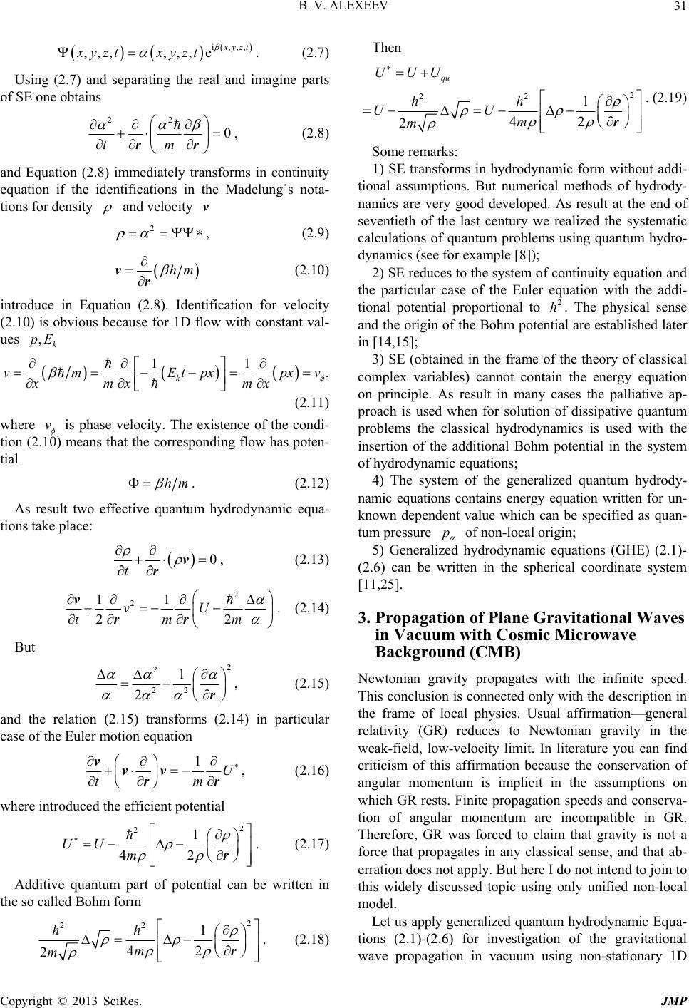 B. V. ALEXEEV 31 ,,, , i,,, ,, e yzt zt xyzt xy . (2.7) Using (2.7) and separating the real and imagine parts of SE one obtains 22 0 tm rr , (2.8) and Equation (2.8) immediately transforms in continuity equation if the identifications in the Madelung’s nota- tions for density and velocity v 2 , (2.9) m r ,k pE v (2.10) introduce in Equation (2.8). Identification for velocity (2.10) is obvious because for 1D flow with constant val- ues px v mx 11 k vmE tpx xmx v , (2.11) where is phase velocity. The existence of the condi- tion (2.10) means that the corresponding flow has poten- tial m . (2.12) As result two effective quantum hydrodynamic equa- tions take place: 0 v r t , (2.13) 2 22 m 2 11 vU tm v rr . (2.14) But 2 22 1 2 2 r , (2.15) and the relation (2.15) transforms (2.14) in particular case of the Euler motion equation 1U tm rr vvv , (2.16) where introduced the efficient potential 2 1 42 r 2 UUm . (2.17) Additive quantum part of potential can be written in the so called Bohm form 2 1 42 r 22 2m m . (2.18) Then 2 22 1 42 2 qu UUU UU m m r 2 p . (2.19) Some remarks: 1) SE transforms in hydrodynamic form without addi- tional assumptions. But numerical methods of hydrody- namics are very good developed. As result at the end of seventieth of the last century we realized the systematic calculations of quantum problems using quantum hydro- dynamics (see for example [8]); 2) SE reduces to the system of continuity equation and the particular case of the Euler equation with the addi- tional potential proportional to . The physical sense and the origin of the Bohm potential are established later in [14,15]; 3) SE (obtained in the frame of the theory of classical complex variables) cannot contain the energy equation on principle. As result in many cases the palliative ap- proach is used when for solution of dissipative quantum problems the classical hydrodynamics is used with the insertion of the additional Bohm potential in the system of hydrodynamic equations; 4) The system of the generalized quantum hydrody- namic equations contains energy equation written for un- known dependent value which can be specified as quan- tum pressure of non-local origin; 5) Generalized hydrodynamic equations (GHE) (2.1)- (2.6) can be written in the spherical coordinate system [11,25]. 3. Propagation of Plane Gravitational Waves in Vacuum with Cosmic Microwave Background (CMB) Newtonian gravity propagates with the infinite speed. This conclusion is connected only with the description in the frame of local physics. Usual affirmation—general relativity (GR) reduces to Newtonian gravity in the weak-field, low-velocity limit. In literature you can find criticism of this affirmation because the conservation of angular momentum is implicit in the assumptions on which GR rests. Finite propagation speeds and conserva- tion of angular momentum are incompatible in GR. Therefore, GR was forced to claim that gravity is not a force that propagates in any classical sense, and that ab- erration does not apply. But here I do not intend to join to this widely discussed topic using only unified non-local model. Let us apply generalized quantum hydrodynamic Equa- tions (2.1)-(2.6) for investigation of the gravitational wave propagation in vacuum using non-stationary 1D Copyright © 2013 SciRes. JMP 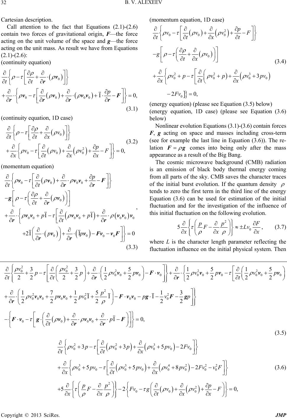 B. V. ALEXEEV Copyright © 2013 SciRes. JMP 32 (momentum equation, 1D case) Cartesian description. Call attention to the fact that Equations (2.1)-(2.6) contain two forces of gravitational origin, F—the force acting on the unit volume of the space and g—the force acting on the unit mass. As result we have from Equations (2.1)-(2.6): (continuity equation) 0 0000 tt v r vvvv rrr I0, p F r (3.1) (continuity equation, 1D case) 0 2 00 v tt x vvv xtx 00, pF x (3.2) (momentum equation) 0000 0 00 00 00 II 2I I p tt t pp t pp vvvv rr gv r vv vv rr vv rr 00 0 00 0 F vv v FvvF , (3.3) 2 000 0 223 0000 0 3 20, p vvvF ttxt gv tx vpvpvpv xtx Fv (3.4) (energy equation) (please see Equation (3.5) below) (energy equation, 1D case) (please see Equation (3.6) below) Nonlinear evolution Equations (3.1)-(3.6) contain forces F, g acting on space and masses including cross-term (see for example the last line in Equation (3.6)). The re- lation g comes into being only after the mass appearance as a result of the Big Bang. The cosmic microwave background (CMB) radiation is an emission of black body thermal energy coming from all parts of the sky. CMB saves the character traces of the initial burst evolution. If the quantum density tends to zero the first term in the third line of the energy Equation (3.6) can be used for estimation of the initial fluctuation and for the investigation of the influence of this initial fluctuation on the following evolution. 2 0 5pp F FLv xx , (3.7) where L is the character length parameter reflecting the fluctuation influence on the initial physical system. Then 22 00 22 000 000 3 3 22 22 171 222 vv p p tt vp vv vv r 22 2 00 00000000 2 2 00 0 151515 2222 22 5 13 2 22 vpvp vp t p pv pv vvFvvv vv rr F vvgFg 00 t Fv gvv 00 0, p p v F rr (3.5) 223 00000 334222 000000 00 2 2 000 3352 5582 52 0, vpvpvpv Fv ttx vpvvpvvpvFvvF xtx pp p FFvgvvF xx txx (3.6) 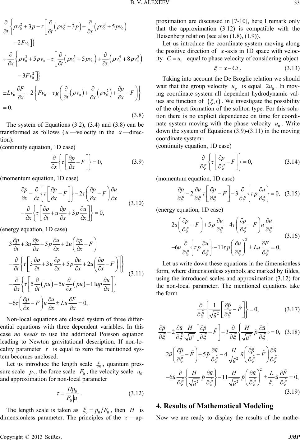 B. V. ALEXEEV 33 22 00 0 33 00 00 2 0 2 00 0 33 2 55 3 2 0. vpvp v tt Fv vpv vpv xt Fv F LvFv gvv xt 3 00 42 00 0 5 8 pv x vpv x p F xx (3.8) The system of Equations (3.2), (3.4) and (3.8) can be transformed as follows (u—velocity in the —direc- tion): (continuity equation, 1D case) 0, pF xx (3.9) (momentum equation, 1D case) 2 pp 30, pu FF tx pp up xtx x x u x (3.10) (energy equation, 1D case) 33 52 33 5 55 60 ppup upu txx x ppu up ttxx pu upu xt x puF Fu Lu xxx 2 11 , F p uF x u up x (3.11) Non-local equations are closed system of three differ- ential equations with three dependent variables. In this case no needs to use the additional Poisson equation leading to Newton gravitational description. If non-lo- cality parameter is equal to zero the mentioned sys- tem becomes unclosed. Let us introduce the length scale 0 , quantum pres- sure scale 0, the force scale 0 p , the velocity scale and approximation for non-local parameter 0 u 0 0 p u . (3.12) The length scale is taken as 000 pF , then is dimensionless parameter. The principles of the —ap- proximation are discussed in [7-10], here I remark only that the approximation (3.12) is compatible with the Heisenberg relation (see also (1.8), (1.9)). Let us introduce the coordinate system moving along the positive direction of -axis in 1D space with veloc- ity 0 Cu equal to phase velocity of considering object Ct . (3.13) Taking into account the De Broglie relation we should wait that the group velocity u2u is equal 0. In mov- ing coordinate system all dependent hydrodynamic val- ues are function of ,t . We investigate the possibility of the object formation of the soliton type. For this solu- tion there is no explicit dependence on time for coordi- nate system moving with the phase velocity 0. Write down the system of Equations (3.9)-(3.11) in the moving coordinate system: u (continuity equation, 1D case) 0, pF (3.14) (momentum equation, 1D case) 230, pup u Fp (3.15) (energy equation, 1D case) 2 254 611 0, pupu uFp Fu uuF upp Lu (3.16) Let us write down these equations in the dimensionless form, where dimensionless symbols are marked by tildes, using the introduced scales and approximation (3.12) for the non-local parameter. The mentioned equations take the form 2 10, pF u (3.17) 22 230, puHp Hu Fp uu (3.18) 2 2 22 0 254 611 0, puHpu uFpuF u HuH uLF upp u uu (3.19) 4. Results of Mathematical Modeling Now we are ready to display the results of the mathe- Copyright © 2013 SciRes. JMP 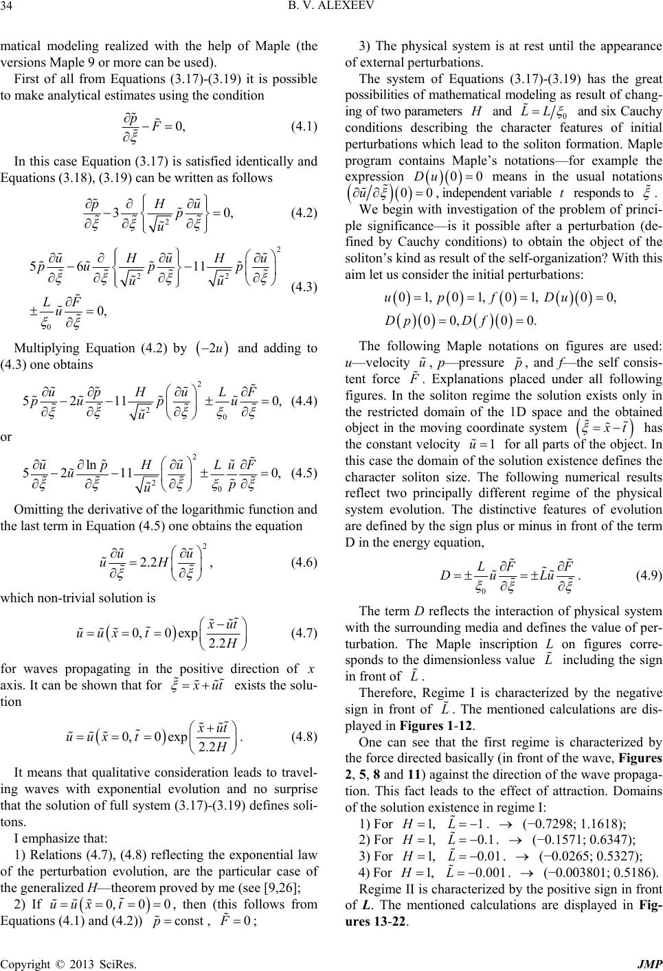 B. V. ALEXEEV 34 matical modeling realized with the help of Maple (the versions Maple 9 or more can be used). First of all from Equations (3.17)-(3.19) it is possible to make analytical estimates using the condition 0, pF (4.1) In this case Equation (3.17) is satisfied identically and Equations (3.18), (3.19) can be written as follows 2 30, u p pH u (4.2) 2 22 11 Hu p u 0 56 0, uHu pu p u LF u 2u (4.3) Multiplying Equation (4.2) by and adding to (4.3) one obtains 2 2 5211 upHu pup u 0 0, LF u (4.4) or 2 2 ln 52 11 upHu uu 0 0, LuF p (4.5) Omitting the derivative of the logarithmic function and the last term in Equation (4.5) one obtains the equation 2 2.2 , uu H u (4.6) which non-trivial solution is 0,0 exp2.2 ut uux t (4.7) for waves propagating in the positive direction of axis. It can be shown that for ut exists the solu- tion 0,0exp2.2 ut uux t 0,0 0t const . (4.8) It means that qualitative consideration leads to travel- ing waves with exponential evolution and no surprise that the solution of full system (3.17)-(3.19) defines soli- tons. I emphasize that: 1) Relations (4.7), (4.8) reflecting the exponential law of the perturbation evolution, are the particular case of the generalized H—theorem proved by me (see [9,26]; 2) If , then (this follows from Equations (4.1) and (4.2)) uux p , ; 3) The physical system is at rest until the appearance of external perturbations. The system of Equations (3.17)-(3.19) has the great possibilities of mathematical modeling as result of chang- ing of two parameters and 0 LL and six Cauchy conditions describing the character features of initial perturbations which lead to the soliton formation. Maple program contains Maple’s notations—for example the expression 00Du means in the usual notations 0F 00u t , independent variable responds to . We begin with investigation of the problem of princi- ple significance—is it possible after a perturbation (de- fined by Cauchy conditions) to obtain the object of the soliton’s kind as result of the self-organization? With this aim let us consider the initial perturbations: 01, 01, 01, 0 0, 00, 00. upf Du Dp Df u p The following Maple notations on figures are used: u—velocity , p—pressure , and f—the self consis- tent force . Explanations placed under all following figures. In the soliton regime the solution exists only in the restricted domain of the 1D space and the obtained object in the moving coordinate system t 1u has the constant velocity for all parts of the object. In this case the domain of the solution existence defines the character soliton size. The following numerical results reflect two principally different regime of the physical system evolution. The distinctive features of evolution are defined by the sign plus or minus in front of the term D in the energy equation, 0 LF F Du Lu L L L 1,H . (4.9) The term D reflects the interaction of physical system with the surrounding media and defines the value of per- turbation. The Maple inscription L on figures corre- sponds to the dimensionless value including the sign in front of . Therefore, Regime I is characterized by the negative sign in front of . The mentioned calculations are dis- played in Figures 1-12. One can see that the first regime is characterized by the force directed basically (in front of the wave, Figures 2, 5, 8 and 11) against the direction of the wave propaga- tion. This fact leads to the effect of attraction. Domains of the solution existence in regime I: 1L 1) For 1,H. (−0.7298; 1.1618); 0.1L 2) For 1,H. (−0.1571; 0.6347); . (−0.0265; 0.5327); 0.01L 1,H 3) For 4) For . (−0.003801; 0.5186). 0.001L Regime II is characterized by the positive sign in front of L. The mentioned calculations are displayed in Fig- ures 13-22. Copyright © 2013 SciRes. JMP 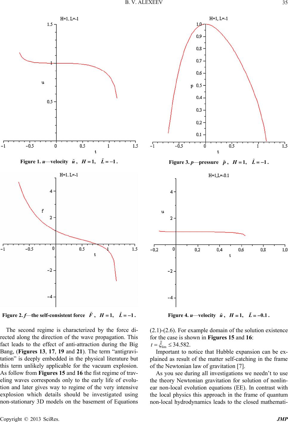 B. V. ALEXEEV 35 Figure 1. u—velocity , . u H1,L 1 Figure 2. f—the self-consistent force , F H1, L 1. The second regime is characterized by the force di- rected along the direction of the wave propagation. This fact leads to the effect of anti-attraction during the Big Bang, (Figures 13, 17, 19 and 21). The term “antigravi- tation” is deeply embedded in the physical literature but this term unlikely applicable for the vacuum explosion. As follow from Figures 15 and 16 the fist regime of trav- eling waves corresponds only to the early life of evolu- tion and later gives way to regime of the very intensive explosion which details should be investigated using non-stationary 3D models on the basement of Equations Figure 3. p—pressure , . p H1, L 1 Figure 4. u—velocity , . u H1,L 0.1 34.582.t (2.1)-(2.6). For example domain of the solution existence for the case is shown in Figures 15 and 16: lim Important to notice that Hubble expansion can be ex- plained as result of the matter self-catching in the frame of the Newtonian law of gravitation [7]. As you see during all investigations we needn’t to use the theory Newtonian gravitation for solution of nonlin- ear non-local evolution equations (EE). In contrast with the local physics this approach in the frame of quantum non-local hydrodynamics leads to the closed mathemati- Copyright © 2013 SciRes. JMP 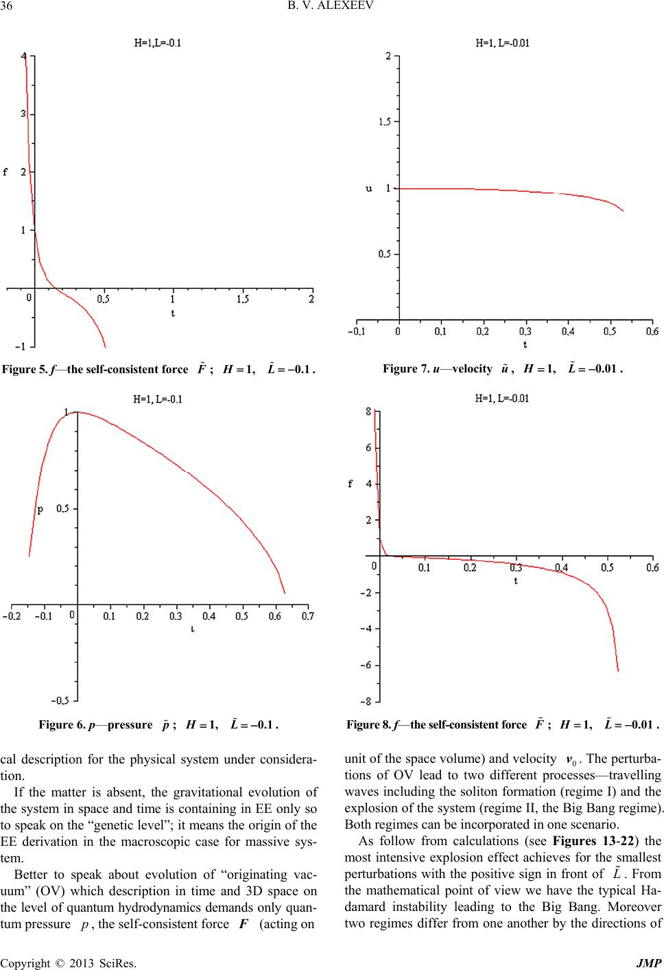 B. V. ALEXEEV 36 Figure 5. f—th e se l f - c o n s i s tent force ; F H1, L 0.1 . Figure 6. p—pressure ; . p H1, L 0.1 pF cal description for the physical system under considera- tion. If the matter is absent, the gravitational evolution of the system in space and time is containing in EE only so to speak on the “genetic level”; it means the origin of the EE derivation in the macroscopic case for massive sys- tem. Better to speak about evolution of “originating vac- uum” (OV) which description in time and 3D space on the level of quantum hydrodynamics demands only quan- tum pressure , the self-consistent force (acting on Figure 7. u—velocity , . u H1, L 0.01 Figure 8. f—the self-consistent force ; . F H1,L 0.01 v L unit of the space volume) and velocity 0. The perturba- tions of OV lead to two different processes—travelling waves including the soliton formation (regime I) and the explosion of the system (regime II, the Big Bang regime). Both regimes can be incorporated in one scenario. As follow from calculations (see Figures 13-22) the most intensive explosion effect achieves for the smallest perturbations with the positive sign in front of . From the mathematical point of view we have the typical Ha- damard instability leading to the Big Bang. Moreover two regimes differ from one another by the directions of Copyright © 2013 SciRes. JMP 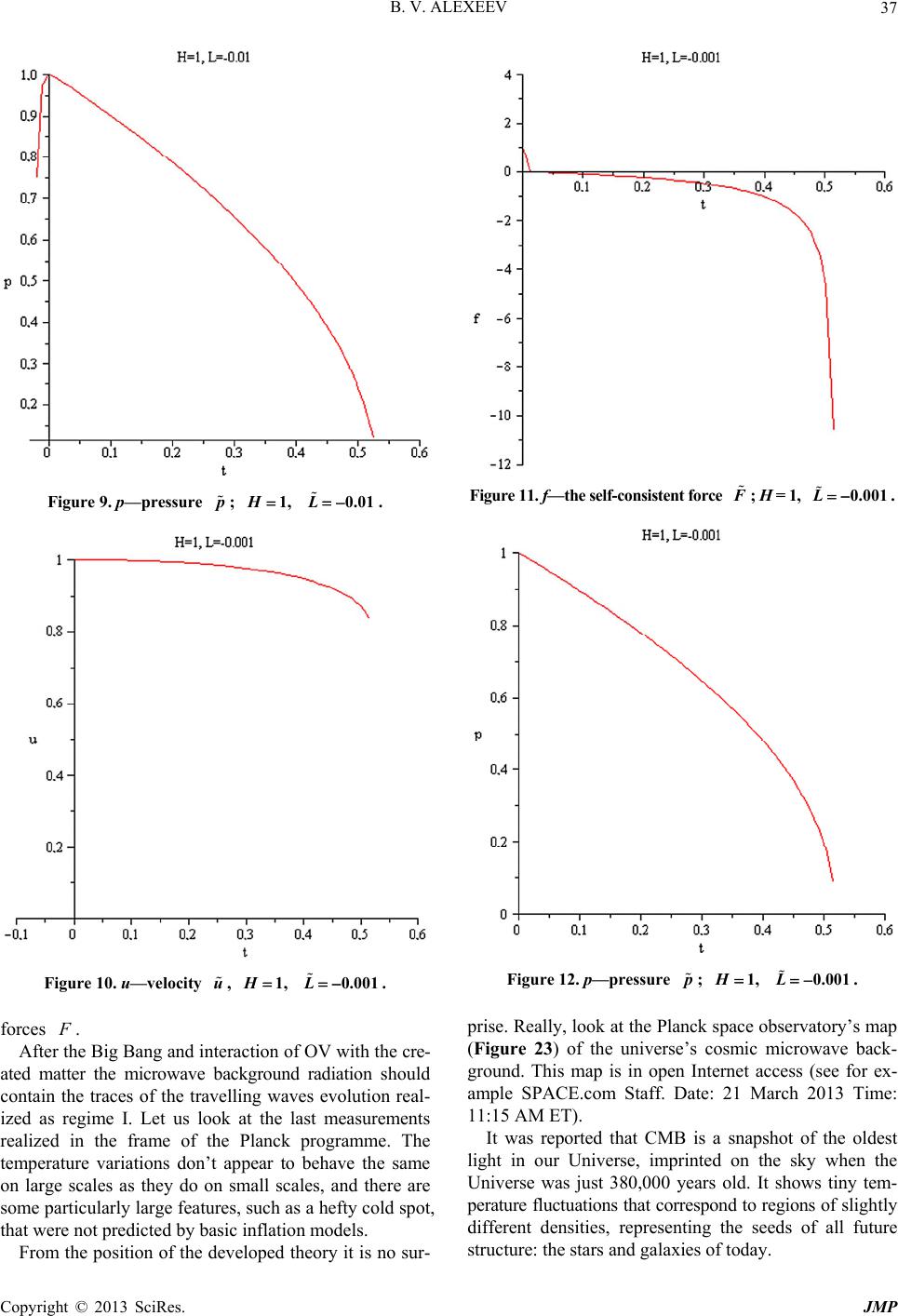 B. V. ALEXEEV 37 Figure 9. p—pressure ; . p H1, L 0.01 Figure 10. u—velocity , . u H1,L 0.001 forces . After the Big Bang and interaction of OV with the cre- ated matter the microwave background radiation should contain the traces of the travelling waves evolution real- ized as regime I. Let us look at the last measurements realized in the frame of the Planck programme. The temperature variations don’t appear to behave the same on large scales as they do on small scales, and there are some particularly large features, such as a hefty cold spot, that were not predicted by basic inflation models. From the position of the developed theory it is no sur- Figure 11. f—the self-consistent force ; H = 1, . F L 0.001 Figure 12. p—pressure H1, L 0.001 ; . prise. Really, look at the Planck space observatory’s map (Figure 23) of the universe’s cosmic microwave back- ground. This map is in open Internet access (see for ex- ample SPACE.com Staff. Date: 21 March 2013 Time: 11:15 AM ET). It was reported that CMB is a snapshot of the oldest light in our Universe, imprinted on the sky when the Universe was just 380,000 years old. It shows tiny tem- perature fluctuations that correspond to regions of slightly different densities, representing the seeds of all future structure: the stars and galaxies of today. Copyright © 2013 SciRes. JMP 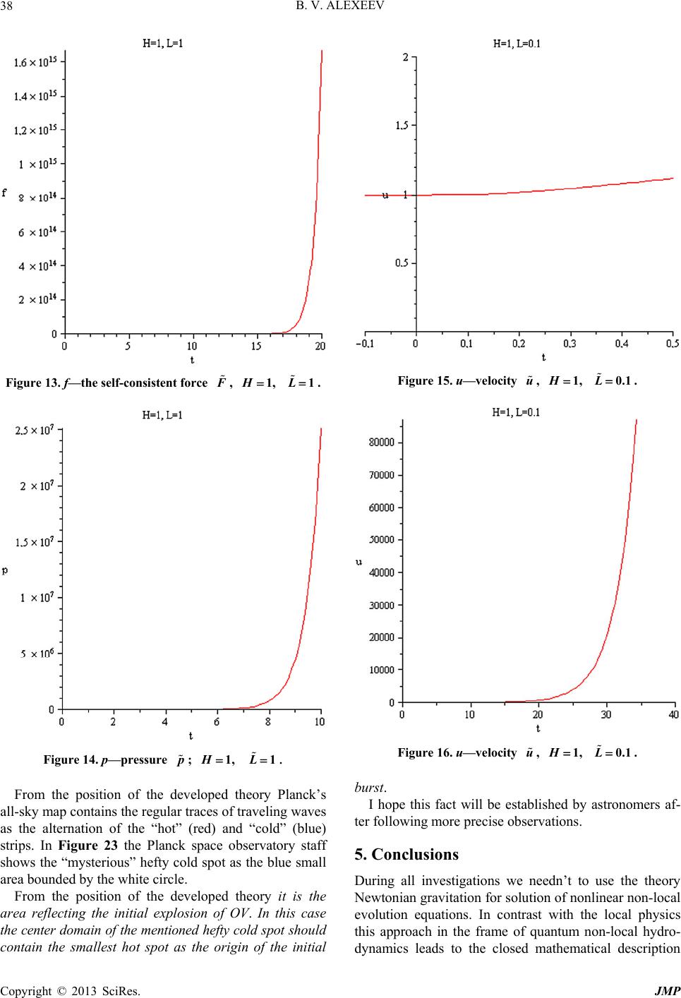 B. V. ALEXEEV 38 Figure 13. f—the self-consistent force , F H1, L 1. Figure 14. p—pressure ; . p H1, L 1 From the position of the developed theory Planck’s all-sky map contains the regular traces of traveling waves as the alternation of the “hot” (red) and “cold” (blue) strips. In Figure 23 the Planck space observatory staff shows the “mysterious” hefty cold spot as the blue small area bounded by the white circle. From the position of the developed theory it is the area reflecting the initial explosion of OV. In this ca s e the center domain of the mentioned hefty cold spot should contain the smallest hot spot as the origin of the initial Figure 15. u—velocity , . u H1,L 0.1 Figure 16. u—velocity , . u H1,L 0.1 burst. I hope this fact will be established by astronomers af- ter following more precise observations. 5. Conclusions During all investigations we needn’t to use the theory Newtonian gravitation for solution of nonlinear non-local evolution equations. In contrast with the local physics this approach in the frame of quantum non-local hydro- dynamics leads to the closed mathematical description Copyright © 2013 SciRes. JMP 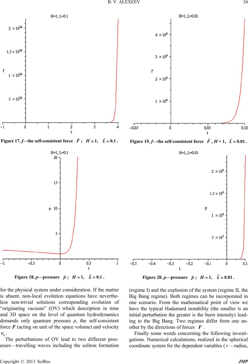 B. V. ALEXEEV 39 Figure 17. f—the self-consistent force ; . F H1, L 0.1 Figure 18. p—pressure ; . p H1,L 0.1 0 v for the physical system under consideration. If the matter is absent, non-local evolution equations have neverthe- less non-trivial solutions corresponding evolution of “originating vacuum” (OV) which description in time and 3D space on the level of quantum hydrodynamics demands only quantum pressure p, the self-consistent force F (acting on unit of the space volume) and velocity . The perturbations of OV lead to two different proc- esses—travelling waves including the soliton formation Figure 19. f—the self-consistent force , H = 1, . F L 0.01 Figure 20. p—pressure H1,L 0.01 F r ; . (regime I) and the explosion of the system (regime II, the Big Bang regime). Both regimes can be incorporated in one scenario. From the mathematical point of view we have the typical Hadamard instability (the smaller is an initial perturbation the greater is the burst intensity) lead- ing to the Big Bang. Two regimes differ from one an- other by the directions of forces . Finally some words concerning the following investi- gations. Numerical calculations, realized in the spherical coordinate system for the dependent variables (—radius, Copyright © 2013 SciRes. JMP 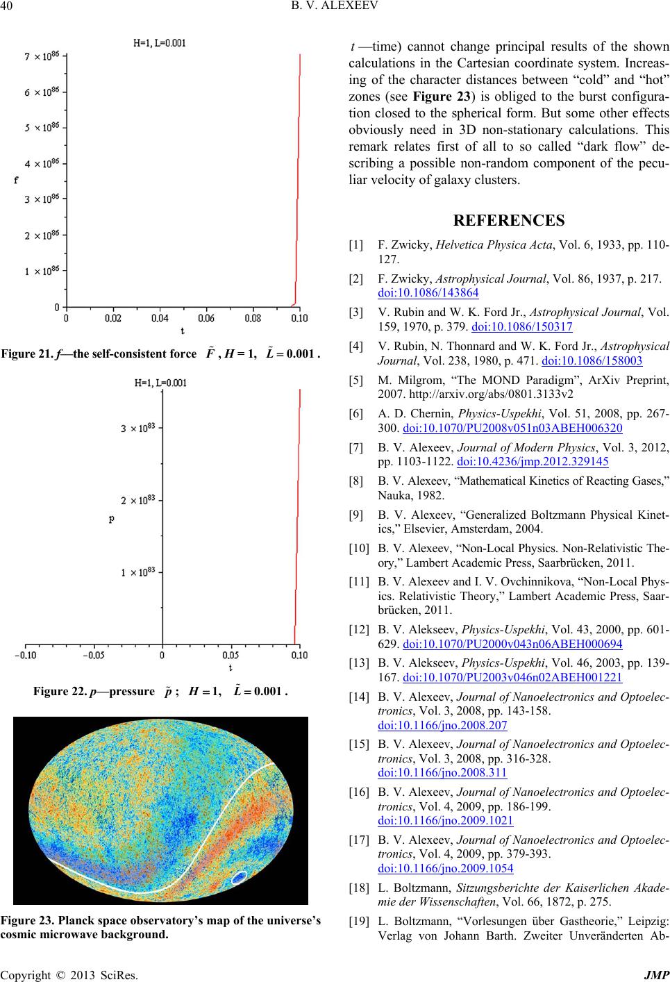 B. V. ALEXEEV 40 t Figure 21. f—the self-consistent force , H = 1, . F L 0.001 Figure 22. p—pressure ; . p H1,L 0.001 Figure 23. Planck space observatory’s map of the universe’s cosmic microw ave background. —time) cannot change principal results of the shown calculations in the Cartesian coordinate system. Increas- ing of the character distances between “cold” and “hot” zones (see Figure 23) is obliged to the burst configura- tion closed to the spherical form. But some other effects obviously need in 3D non-stationary calculations. This remark relates first of all to so called “dark flow” de- scribing a possible non-random component of the pecu- liar velocity of galaxy clusters. REFERENCES [1] F. Zwicky, Helvetica Physica Acta, Vol. 6, 1933, pp. 110- 127. [2] F. Zwicky, Astrophysical Journal, Vol. 86, 1937, p. 217. doi:10.1086/143864 [3] V. Rubin and W. K. Ford Jr., Astrophysical Journal, Vol. 159, 1970, p. 379. doi:10.1086/150317 [4] V. Rubin, N. Thonnard and W. K. Ford Jr., Astrophysical Journal, Vol. 238, 1980, p. 471. doi:10.1086/158003 [5] M. Milgrom, “The MOND Paradigm”, ArXiv Preprint, 2007. http://arxiv.org/abs/0801.3133v2 [6] A. D. Chernin, Physics-Uspekhi, Vol. 51, 2008, pp. 267- 300. doi:10.1070/PU2008v051n03ABEH006320 [7] B. V. Alexeev, Journal of Modern Physics, Vol. 3, 2012, pp. 1103-1122. doi:10.4236/jmp.2012.329145 [8] B. V. Alexeev, “Mathematical Kinetics of Reacting Gases,” Nauka, 1982. [9] B. V. Alexeev, “Generalized Boltzmann Physical Kinet- ics,” Elsevier, Amsterdam, 2004. [10] B. V. Alexeev, “Non-Local Physics. Non-Relativistic The- ory,” Lambert Academic Press, Saarbrücken, 2011. [11] B. V. Alexeev and I. V. Ovchinnikova, “Non-Local Phys- ics. Relativistic Theory,” Lambert Academic Press, Saar- brücken, 2011. [12] B. V. Alekseev, Physics-Uspekhi, Vol. 43, 2000, pp. 601- 629. doi:10.1070/PU2000v043n06ABEH000694 [13] B. V. Alekseev, Physics-Uspekhi, Vol. 46, 2003, pp. 139- 167. doi:10.1070/PU2003v046n02ABEH001221 [14] B. V. Alexeev, Journal of Nanoelectronics and Optoelec- tronics, Vol. 3, 2008, pp. 143-158. doi:10.1166/jno.2008.207 [15] B. V. Alexeev, Journal of Nanoelectronics and Optoelec- tronics, Vol. 3, 2008, pp. 316-328. doi:10.1166/jno.2008.311 [16] B. V. Alexeev, Journal of Nanoelectronics and Optoelec- tronics, Vol. 4, 2009, pp. 186-199. doi:10.1166/jno.2009.1021 [17] B. V. Alexeev, Journal of Nanoelectronics and Optoelec- tronics, Vol. 4, 2009, pp. 379-393. doi:10.1166/jno.2009.1054 [18] L. Boltzmann, Sitzungsberichte der Kaiserlichen Akade- mie der Wissenschaften, Vol. 66, 1872, p. 275. [19] L. Boltzmann, “Vorlesungen über Gastheorie,” Leipzig: Verlag von Johann Barth. Zweiter Unveränderten Ab- Copyright © 2013 SciRes. JMP 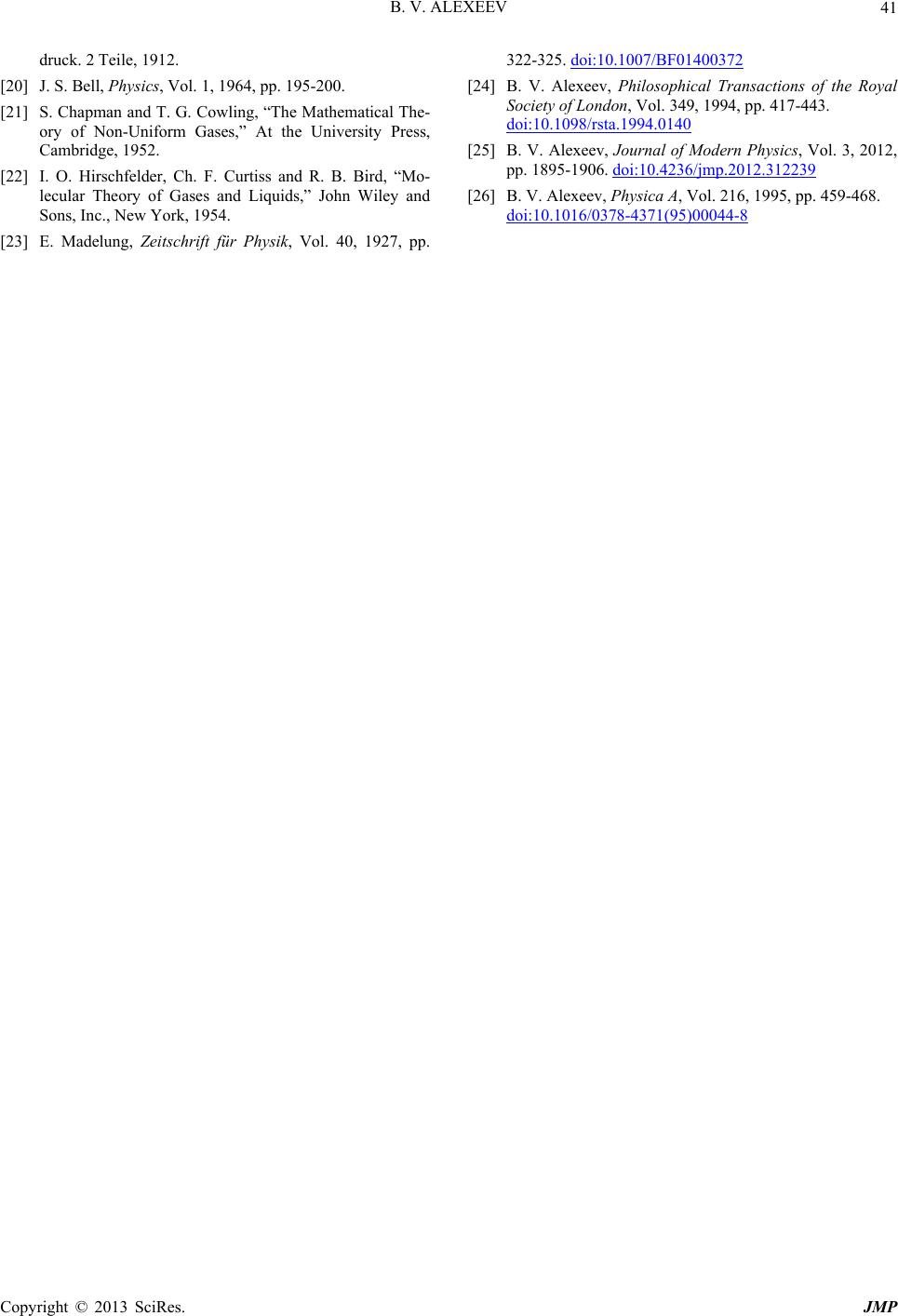 B. V. ALEXEEV Copyright © 2013 SciRes. JMP 41 druck. 2 Teile, 1912. [20] J. S. Bell, Physics, Vol. 1, 1964, pp. 195-200. [21] S. Chapman and T. G. Cowling, “The Mathematical The- ory of Non-Uniform Gases,” At the University Press, Cambridge, 1952. [22] I. O. Hirschfelder, Ch. F. Curtiss and R. B. Bird, “Mo- lecular Theory of Gases and Liquids,” John Wiley and Sons, Inc., New York, 1954. [23] E. Madelung, Zeitschrift für Physik, Vol. 40, 1927, pp. 322-325. doi:10.1007/BF01400372 [24] B. V. Alexeev, Philosophical Transactions of the Royal Society of London, Vol. 349, 1994, pp. 417-443. doi:10.1098/rsta.1994.0140 [25] B. V. Alexeev, Journal of Modern Physics, Vol. 3, 2012, pp. 1895-1906. doi:10.4236/jmp.2012.312239 [26] B. V. Alexeev, Physica A, Vol. 216, 1995, pp. 459-468. doi:10.1016/0378-4371(95)00044-8
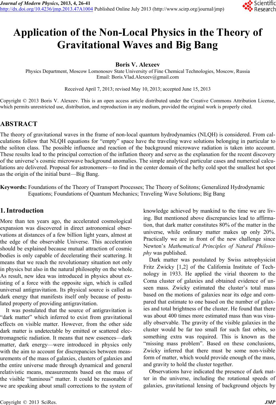
|