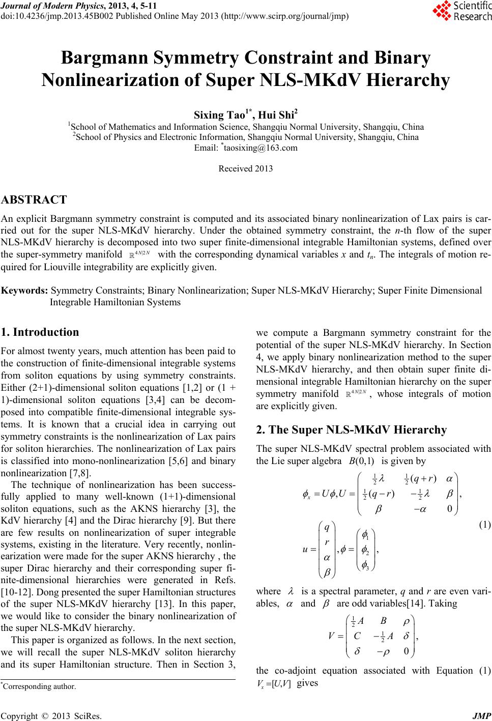
 Journal of Modern Physics, 2013, 4, 5-11 doi:10.4236/jmp.2013.45B002 Published Online May 2013 (http://www.scirp.org/journal/jmp) Bargmann Symmetry Constraint and Binary Nonlinearization of Super NLS-MKdV Hierarchy Sixing Tao1*, Hui Shi2 1School of Mathematics and Information Science, Shangqiu Normal University, Shangqiu, China 2School of Physics and Electronic Information, Shangqiu Normal University, Shangqiu, China Email: *taosixing@163.com Received 2013 ABSTRACT An explicit Bargmann symmetry constraint is computed and its associated binary nonlinearization of Lax pairs is car- ried out for the super NLS-MKdV hierarchy. Under the obtained symmetry constraint, the n-th flow of the super NLS-MKdV hierarchy is decomposed into two super finite-dimensional integrable Hamiltonian systems, defined over the super-symmetry manifold with the corresponding dynamical variables x and tn. The integrals of motion re- quired for Liouville integrability are explicitly given. 4|2 NN Keywords: Symmetry Constraints; Binary Nonlinearization; Super NLS-MKdV Hierarchy; Super Finite Dimensional Integrable Hamiltonian Systems 1. Introduction For almost twenty years, much attention has been paid to the construction of finite-dimensional integrable systems from soliton equations by using symmetry constraints. Either (2+1)-dimensional soliton equations [1,2] or (1 + 1)-dimensional soliton equations [3,4] can be decom- posed into compatible finite-dimensional integrable sys- tems. It is known that a crucial idea in carrying out symmetry constraints is the no nlinearization of Lax pairs for soliton hierarchies. The nonlinearization of Lax pairs is classified into mono-nonlinearization [5,6] and binary nonlinea r i zation [7,8] . The technique of nonlinearization has been success- fully applied to many well-known (1+1)-dimensional soliton equations, such as the AKNS hierarchy [3], the KdV hierarchy [4] and the Dirac hierarchy [9]. But there are few results on nonlinearization of super integrable systems, existing in the literature. Very recently, nonlin- earization were made for the super AKNS hierarchy , the super Dirac hierarchy and their corresponding super fi- nite-dimensional hierarchies were generated in Refs. [10-12]. Dong presented the super Hamiltonian structures of the super NLS-MKdV hierarchy [13]. In this paper, we would like to consider the binary nonlinearization of the super NLS- M Kd V hierarchy. This paper is organized as follows. In the next section, we will recall the super NLS-MKdV soliton hierarchy and its super Hamiltonian structure. Then in Section 3, we compute a Bargmann symmetry constraint for the potential of the super NLS-MKdV hierarchy. In Section 4, we apply binary nonlinearization method to the super NLS-MKdV hierarchy, and then obtain super finite di- mensional integrable Hamiltonian hierarchy on the super symmetry manifold , whose integrals of motion are explicitly given. 4|2 NN 2. The Super NLS-MKdV Hierarchy The super NLS-MKdV spectral problem associated with the Lie super algebra is given by (0,1)B 11 22 11 22 1 2 3 () ,() 0 ,, x qr UU qr q r u , (1) where is a spectral parameter, q and r are even vari- ables, and are odd var i ables[14]. Taking 1 2 1 2, 0 AB VC A the co-adjoint equation associated with Equation (1) [,] x VUV gives *Corresponding author. Copyright © 2013 SciRes. JMP  S. X. TAO, H. SHI. 6 1 2 1 2 ()()22 ()2, ()2, 22( 22( x x x x x AqrBqrC BBqrA CCqrA ABqr ACqr , ), ). , i i (2) If we set 000 00 ,, ,, ii ii iii ii ii ii AABBCC (3) then Equation (2) is equivalent to 1 1, 2 1 1, 2 1, 1, 1,111 1 () 2, () 2, 22(), 2()2, ()()2 2, iiixi iiixi iiiix i iii iix ixiii i BqrAB CqrAC AB qr ACqr AqrBqrC i 0. (4) which results in the recurrence relations T 11111 1 T 1 (,,4,4) (,,4,4), (()() 22),0. iiiii i iiiii i iiiiiii BCCB LBC CB AqCBrBC i (5) where Upon choosing the initial conditions 0000 0 0, 1,BC A all other ,,,,( 1) iiiii ABC i can be worked out by the recurre n c e r e l ations Equation (5). The fir s t few sets a re : 11 11 1 22 22 11 11 2 22 11 11 22 22 22 22 32 2 1111 1 32244 4 3 1 4 32 2 1111 1 32244 4 0,( ),( ), ,, 4, ,, 2, 2, 4 22, 4 xx xx xx xx xxx xx xxx ABqrCqr Aqr BqrC qr Bq rqqrqr rq r Cqrqqrqr 3 1 4 22 11 322 22 11 322 22, 422 422 xx xxxx xx xxxx rq r qr qrqr qr qrqr 388. xx Aqrqr x Let us associate the spectral problem Equation (1) with the following aux iliary problem () () n nn tVV, (7) with 1 2 () 1 2 0, 0 iii n nn iii i ii AB VCA i where the symbol “ ” denotes taking the non-negative part in the power of . The compatible conditions of the spectral problem Equation (1) and th e auxiliary problem Equation (7) are () () [,]0, n nn tx UV UV (8) which infer the super NLS-MKdV hierarchy T 11 11111 1 22 (,,, 0. n tnnnnnn n uK BCBC n ), (9) Here in Equation (9) is called the n-th NLS –MKdV flow of this hierarchy. n n t uK Using the super trace identity StrdStr, UU Vx V uu (10) where Str means the super trace [14,15], we have 11 11 2 1 1 ,d, 41 4 ii ii i ii i i BC CB A HH xi ui 0. (11) Therefore, the super NLS-MKdV soliton hierarchy Equation (9) can be written as the following super Ham- iltonian for m: , n n t uJ u (12) where , , 1 8 1 8 0100 10 00 . 000 00 0 J is a super symplectic operator, and n is given by Equation (11). 111 11 22 1111 11 22 11 11 111 ()( ()() . 44 44222 44 44222 qrqq qq rr rqrr Lrq rqqr 1 1 ) qr (6) Copyright © 2013 SciRes. JMP  S. X. TAO, H. SHI 7 The first non-trivial nonlinear equation of the super NLS-MKdV hierarcy (9) is given by its second flow 2 2 2 2 23 11 22 32 11 22 22 11 11 22 44 22 11 11 22 44 44 4, 44 4, 2, 2. txxx x txxx x txxxx xx txxxxxx qrqrr r rqq qr q qrqrqr qrqrqr (13) which possesses a Lax pair of U defined in Equation (1) and defined by (2) V 3. Bargmann Symmetry Constraint of Super NLS-MKdV Hierarchy In order to compute a Bargmann symmetry constraint, we consider the following adjoint spectral problem of the spectral problem: 11 1 22 11 2 22 3 () () , 0 St x qr Uqr , (15) where means the super transposition. The following result is a general formula for the variational derivative with respect to the potential u (see[3] for the classical case). St Lemma 1 [10-12] Let (, )Uu be an even matrix of order depending on and a parame- ter mn,,uu ,, xxx u . Suppose tha t T (,) eo and satisfy the spectral problem and the adjoint spectral problem T (, eo ) (, ),, St xx Uu U (16) where 1,, em and 1,, em ,, om mn om are even eigenfunctions, and and ,,mn are odd eigenfunctions. Then the variational derivative of the parameter with respect to the potential u is given by () ,( 1), d pu U eo u TU ux (17) where we denote 0, , () 1, . v is aneven variable pv v isan oddvariable (18) By Lemma 1, it is not difficult to find that 11 12 21 22 11 12 21 22 13 32 23 31 1. uE (19) where 1112 2 2(E )d.x If we consider zero boundary conditions || || lim lim0, xx we can obtain a characteristic property- a recurrence relation for the variational derivative of : ,Luu (20) where L and u are given by Equation (4) and Equation (18), respectively. Let us now discuss the spatial systems: 11 11 22 11 22 22 33 11 11 22 11 22 22 33 () () , 0 () () 0 jj jj jj x jj jj jj x qr qr qr qr , (21) and the temporal systems: 222 11111 24422 (2)22 2 11 111 22 244 2()() 2 () ()22 22 xx x xx x xx qrqrqr Vqrqrqr . 0 (14) 1 2 000 1 1 1 2 2 2 000 3 3 00 1 2 0 1 2 3 , 0 n n nnn ni ni ni ij ij ij iii j j nnn nini ni jij ijij iii nn ni ni j j tij ij ii nni n ij ij i j j jt AB CA AC j 00 1 12 2 00 0 3 00 , 0 nn ini ij iij nn n nini ni ijijij j ii i nn ni nij ij ij ii BA (22) Copyright © 2013 SciRes. JMP  S. X. TAO, H. SHI. 8 where and 12 1jN ,,,N are N distinct pa- rameters. Now for systems Equation (21) and Equation (22), we have the following symm e try constraints: 1,0. (23) Nj kj j Hk uu The symmetry constraints in the case of 0k is called a Bargmann constraint (see[8]). If taking ij E 1112 2 2( jjj j )d , then it leads to an expression for the potential , i.e. u 112 21 2 121 12 2 123 31 4 113 32 4 ,, ,, ,, ,, q r , , , , (24) where we use the following notation TT 11 ,,,,,, 1,2,3. iiiNiiiN i and , denotes the standard inner product of the Euclidean space . 4. Binary Nonlinearization of Super NLS –MKdV Hierarchy In order to perform binary nonlineqrization to the super NLS-MKdV hierarchy. To this end, let us substituting Equation (24) into the Lax pairs and adjoint Lax pairs Equa- tion (21) and Equation (22), and then we obtain the follow- ing nonlinearized spatial Lax pairs and adjoint Lax pairs: 11 11 22 11 22 22 33 11 11 22 11 22 22 33 () (), 0 () () 0 jj jj jj x jj jj jj x qr qr qr qr , (25) and where 1jN and means an expression of under the explicit constraint Equation (24). Note that the spatial part of the nonlinearized system Equation (25) is a system of ordinary differential equations with an inde- pendent variables u, but for a given , the - part of the nonlinearized system Equation (26) is a sys- tem of ordinary differential equations. Obviously, the system Equation (25) can be written as P()Pu n t(2nn) where 1 diag( ,,).N When , the system Equation (26) is exactly the system Equation (25) with 1 1n tx . The system Equation (25) or Equation (27) can be written as the following super Hamiltonian form: 111 1, 2,3, 12 11 1, 2,3, 12 ,, ,, xxx xxx HHH 3 1 3 , . HH (28) where 11 1 11122233 22 4 13 32 ,,, ,,. H 1 , 1 2 000 1 1 1 2 2 2 000 3 3 00 1 2 1 2 3 , 0 n n nnn ni ni ni ij ij ij iii j j nnn nini ni jij ijij iii nn ni ni j j tij ij ii ni ij i j j jt AB CA A j 000 1 12 2 00 0 3 00 , 0 nnn ni ni ij ij iij nn n nini ni ijijij j iii nn ni nij ij ij ii C BA (26) 111 1,12 12233 13 22 4 111 2,1 21213323 224 11 3,133 2123312 44 111 1,11 221 3323 224 111 2,211223313 224 1 3,2 3 4 ,,, ,,, ,, ,, ,,, ,, , x x x x x x , , , , ,, 1 31 113322 4 ,,, , (27) Copyright © 2013 SciRes. JMP  S. X. TAO, H. SHI 9 When , the system Equation (26) is 2n 2 2 2 2 222 1111 1 1,1 2 2442 2 3 222 11 111 2, 12 22 244 3 3,1 2 2 1 1 1, 24 2()() 2, () ()2 2, 22, txx x txx x tx x t qrqrqr qrq rqr 2 2 22 111 12 422 3 222 11 111 2,1 2 22 244 3 3,1 2 2()() 2, () ()2 2, 22, xx x txx x tx x qrqrqr qrq rqr (29) where ,, , qr , and ,, , xxx qr denote the functions ,, ,qr defined by the explicit constraint Equation (24) are given by 111 211212211122 224 111 21121221 1122 224 111 2331112223 31 8816 11 1 133211 22 13 32 8816 ,,,,,, ,,,,,, ,,,,,, ,,,,,, x x x x q r , , , . (30) re compuatial con (27). The system Equation (29) can be represented as the following super Hamiltonian form: which ated through using the spstrained flow Equation 222 222 22 1, 2,3, 12 22 1, 2, 3, 12 2 3 2 ,,, ,,. ttt ttt HHH 3 HH (31) where 22 11 211 22 22 1 ,, ,,, 21 12 1122 4 123311332 8 112 2 11 21 122112 22 123311332 4 123 3 4 , ,,,, ,, +,,,, ,, ,, ,, H 11332 ,,. In what follows, we want to prove that Equation (25) is a completely integrable Hamiltonian system in the Liouville sense. Furthermore, we shall prove that Equa- tion (26) is also completely integrable under the contron of system Equation (25). quation (20 and the recurrence relations Equation (5) ensure that In addition, the characteristic property E) 1 11111 2 1 121 2 1 112 2 1 12331 4 1 11332 4 ,,, ,, 0, ,, 0, ,,, 0, ,,, 0. ii i i i i i ii i ii i Ai Bi Ci i i 0, (32) Then the co-adjoint representation equation remains true. Furthermore, we know that also true. Let [,] x VUV 22 [, ] VUV is x 2 Str. V (33) Then it is easy to find that That is easy to see, F is a generating function off motion for the system Equation (25) or Equation (27). Due to 0. x F integrals o 0, n n n FF we obtain the following formulas of integrals of motion: 2 1 00101 2 11 ,, n FAFAA 02 124 ,2. nn iniiniini i FA AAABCi (34) Copyright © 2013 SciRes. JMP  S. X. TAO, H. SHI. 10 Substituting Equation (32) into the above formulas of motion, we obtain the following expression of ) (0 m Fm: 11 01 1122 22 1 21122 2 12112 2 123311332 4 ,,,, ,, ,, ,,,,, FF F (35) 11 1 11 111 8 1122 2 111 121 12 2 1 1 ,, nin i i n 2 2 , 1 11 11 23 3 4 1 ,, , ,, nn n ii i F 2 2 111 1 ,, i ni ni nii 1 113 , ni 132 ,, ni 2.n On the other hand, let us consider the temporal pa the nonlinearized system Equation (26). Making use of Equation (32) and Equation (36), the system Equation (2 (36) rt of 6) can be written as the following super Hamiltonian form: 11 1, 2, 3, 12 11 1, 2, 3, 12 ,, ,, nnn nnn nn ttt nn ttt FFF FF 1 3 1 3 , . n n F (37) This can be checked pretty easily. For example, we can show one equality in the above system as follows: 1 1,1 23 2 000 11 11 11122 24 1 1 121 2 21 11 12331 3 41 1 1 ,, , ,, =. n nnn ninini ti ii iii n ni i i nini i niini i n AB F 1 ni (38) In order to show the Liouville integrability for the constrained flows Equation (25) and Equation (26), we need to prove the commutative propertity of motion 0 {} mm F, under the corresponding Poission bracket 3()( ) 11 {,}(1) . ij ij Npp ij ijijij ij GF FG G (39) At this time, we still have an equality ] and after a similar discussion, we know that () [, n n t VVV, is also a he hich implies ge system Equatior Equation (37), w nerating function of integrals of motion for Equation (26). Hence 0 {} mm F are integrals of motion for t n (26) o 11 1 {,}0,,0 mn m n FFF mn t . (40) The above equality Equation (40) shows that are in involution in pair under the Poission brac tion (39). In addition, similar to the method in [16], we know that 0 {} mm F ket Equa- 112 23 3 ,1 . kkkkkkk kN (41) are integrals of motion for Equation (25) and Equation (26). It is not difficult to verify that the fun 3Nctions 2 {} 1 mm F and 1 {} kk f are involution in pair. Similar to the methods in [10,16,17], we can verify that the 3Nfunctions 21 {} mm F and 1 {} kk f are functionally independent over some region of the super symmetry 4|2 NN . Now, all of above analysis givemanifold s the following theorem. Theorem 1 Both the spatial and temporal flows tion (25) and Equation (26) are Liouville integrable su- peuper symmetr Equa- r Hamiltonian systems defined on the sy manifold 4|2 N, which possess 3N functionally in- dependent and involutive integrals 21 {} N mm F and 1 {} kk f defined by Equ6) and Equation (41). ation (3 5. Acknowledgements This work was supported by the Natural Science Founda- tiod Tech REFERENCES n of China ( No. 61072147), the Science an- nology Key Research Foundation of Provincial Educa- tion Department of Henan (No. 12A110017), the Youth Research Foundation of Shangqiu Normal University (No. 2011 QN 1 2) . [1] Y. Cheng and Y. S. Li, “The Constraint of The Ka- domtsev-Petviashvili Equation and Its Special Solutions,” Physics Letters A , Vol. 157, No. 1, 1991, pp. 22-26. doi: 10.1016/0375-9601(91)90403-U [2] Y. Cheng, “Constraints of the Kadomtsev-Petviashvili Hierarchy,” Journal of Mathematical Physics, Vol. 33, No. 11, 1992, pp. 3774-3782. doi: 10.1063/1.529875 [3] W. X. Ma and W Strampp, “An Explicit Symmetry Con- straint for the Lax Pairs of AKNS Systems,” Physics Let- ters A, Vol. 185, No. 3, 1994, pp. 277-286. Copyright © 2013 SciRes. JMP  S. X. TAO, H. SHI Copyright © 2013 SciRes. JMP 11 doi: 10.1016/0375-9601(94)90616-5 [4] W. Xew Finite-DimensioIntegrable Systems by Symmetry Constraint of the Kdations,” l of the Physical Society of Japan, Vol. 64, No. 4, 1. 1085-1091. . Ma, “Nnal V EquJourna 995, pp doi: 10.1143/JPSJ.64.1085 [5] Y. B. Zeng and Y. S. Li, and the Finite-Dimensiona“The Constraints of Potentials l Integrable Systems,” Journal of Mathematical Physics, Vol. 30, No. 8, 1989, pp.1679- -1689. doi:10.1063/1.528253 [6] C. W. Cao and X. G. Geng, “A Monconfocal Generator of Involutive Systems and Three Associated Soliton Hi- erarchies,” Journal of Mathematical Physics, Vol. 2, No. 9, 1991, pp. 2323-2328. doi:10.1063/1.529156 [7] W. X. Ma, “Symmetry Constraint of MKdV Equations by Binary Nonlinearization,” Physica A, Vol. 219, No. 3-4, 1995, pp. 467-371(95)00161-Y 481. doi:10.1016/0378-4 [8] W. X. Ma and R. G. Zhou, “Adjoint Symmetry Con- straints Leading to Binaary Nonlinearization,” Journal of Nonlinear Mathematical Physics, Vol. 9, No. Suppl. 1, 2002, pp. 106-126. [9] W. X. Ma, “Binary Bonlinearization for the Dirac Sys- tems,” Chinese Annals of Mathematics, Series B, Vol. 18, No. 1, 1997, pp. 79-88. [10] J. S. He, J. Yu, Y. Cheng and R. G. Zhou, “Binary Bon linearization of the Super AKNS System,” Modern Phys- ics Letters B, Vol. 22, No. 4, 2008, pp. 275-288. doi:10.1142/S0217984908014778 [11] J. Yu, J. W. Han and J. S. He, “Binary Nonlinearization of the Super AKNS System under an Implicit Symmetry constraint,” Journal of Physics A: Mathematical and Theoretical, Vol. 42, No. 46, 2009, 465201. doi:10.1088/1751-8113/42/46/465201 [12] J. Yu, J. S. He, W. X. Ma and Y. Cheng, “The Bargmann 0, pp. 361-372. Symmetry Constraint and Binary Nonlinearization of the Super Dirac System,” Chinese Annals of Mathematics, Series B, Vol. 31, No. 3, 201 doi:10.1007/s11401-009-0032-6 [13] H. H. Dong and X. Z. Wang, “Lie Algebra and Lie Super Algebra for the Integrable Couplings of NLS-M erarchy,” Communications in NoKdV Hi- nlinear Science and Numeical Simulation, Vol. 14, No. 12, 2009, pp. 4071-4077. doi:10.1016/j.cnsns.2009.03.010 [14] W. X. Ma, J. S. He and Z. Y. Qin, “A Supertrace Identity and Its Applications to Super Integrable Syst nal of Mathematical Physics, Vol. ems,” Jour- 49, No. 3, 2008, 033511. doi:10.1063/1.2897036 [15] X. B. Hu, “An Approach to Generate Superextensions of Integrable Systems,” Journal of Physics A: Mathematical and General, Vol. 30, No. 2, 1997, pp. 619-632. doi:10.1088/0305-4470/30/2/023 [16] W. X. Ma, B. Fuchssteiner and W. Oevel, “A 3×3 Matrix Spectral Problem for AKNS Hierarchy and Its Binary Nonlinearization,” Physica A, Vol. 233, No. 1-2, 1996, pp. 331-354. doi: 10.1016/S0378-4371(96)00225-7 [17] W. X. Ma and Z. X. Zhou, “Binary Symmetry Constraints of N-wave Intersection Equations in 1+1 and 2+1 Dimen- sions,” Journal of Mathematical Physics, Vol. 42, No. 9, 2001, pp. 4345-4382. doi:10.1063/1.1388898
|