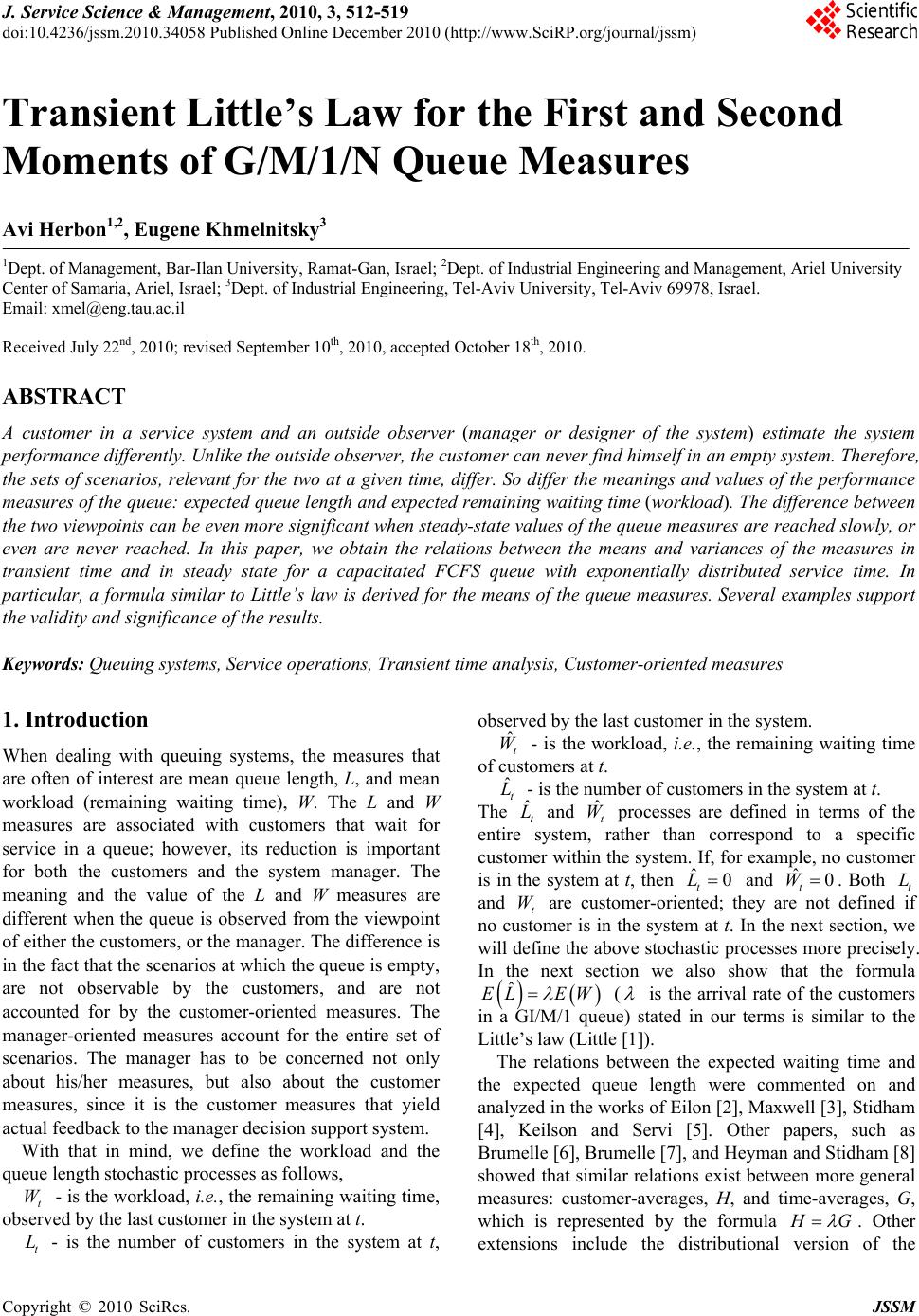J. Service Science & Management, 2010, 3, 512-519
doi:10.4236/jssm.2010.34058 Published Online December 2010 (http://www.SciRP.org/journal/jssm)
Transient Little’s Law for the First and Second
Moments of G/M/1/N Queue Measures
Avi Herbon1,2, Eugene Khmelnitsky3
1Dept. of Management, Bar-Ilan University, Ramat-Gan, Israel; 2Dept. of Industrial Engineering and Management, Ariel University
Center of Samaria, Ariel, Israel; 3Dept. of Industrial Engineering, Tel-Aviv University, Tel-Aviv 69978, Israel.
Received July 22nd, 2010; revised September 10th, 2010, accepted October 18th, 2010.
ABSTRACT
A customer in a service system and an outside observer (manager or designer of the system) estimate the system
performance differently. Unlike th e outside observer, the cu stom er can n ever fin d himself in a n emp ty system. Therefore,
the sets of scenarios, relevant for the two at a given time, differ. So differ the mean ings and values of the performance
measures of the queue: expected queue length and expected remaining waiting time (work l oad). The difference between
the two viewpoints can be even more significan t when steady-state values of th e queue measures ar e reached slowly, or
even are never reached. In this paper, we obtain the relations between the means and variances of the measures in
transient time and in steady state for a capacitated FCFS queue with exponentially distributed service time. In
particular, a formula similar to Little’s law is derived for the means of the queue measures. Several examples support
the validity and significance of th e results.
Keywords: Queuing systems, Service operations, Transient time analysi s, C usto mer- oriented measures
1. Introduction
When dealing with queuing systems, the measures that
are often of interest are mean queue length, L, and mean
workload (remaining waiting time), W. The L and W
measures are associated with customers that wait for
service in a queue; however, its reduction is important
for both the customers and the system manager. The
meaning and the value of the L and W measures are
different when the queue is observed from the viewpoint
of either the customers, or the manager. The difference is
in the fact that the scenarios at which the queue is empty,
are not observable by the customers, and are not
accounted for by the customer-oriented measures. The
manager-oriented measures account for the entire set of
scenarios. The manager has to be concerned not only
about his/her measures, but also about the customer
measures, since it is the customer measures that yield
actual feedback to the manager decision support system.
With that in mind, we define the workload and the
queue length stochastic processes as follows,
t - is the workload, i.e., the remaining waiting time,
observed by the last customer in the system at t.
W
t
L - is the number of customers in the system at t,
observed by the last customer in the system.
ˆt
W - is the workload, i.e., the remaining waiting time
of customers at t.
ˆt
L - is the number of customers in the system at t.
The and processes are defined in terms of the
entire system, rather than correspond to a specific
customer within the system. If, for example, no customer
is in the system at t, then and . Both t
and t are customer-oriented; they are not defined if
no customer is in the system at t. In the next section, we
will define the above stochastic processes more precisely.
In the next section we also show that the formula
ˆt
L
W
ˆt
W
ˆ0
t
Lˆ0
t
WL




W
ˆ
EL E  (

is the arrival rate of the customers
in a GI/M/1 queue) stated in our terms is similar to the
Little’s law (Little [1]).
The relations between the expected waiting time and
the expected queue length were commented on and
analyzed in the works of Eilon [2], Maxwell [3], Stidham
[4], Keilson and Servi [5]. Other papers, such as
Brumelle [6], Brumelle [7], and Heyman and Stidham [8]
showed that similar relations exist between more general
measures: customer-averages, H, and time-averages, G,
which is represented by the formula
H
G

. Other
extensions include the distributional version of the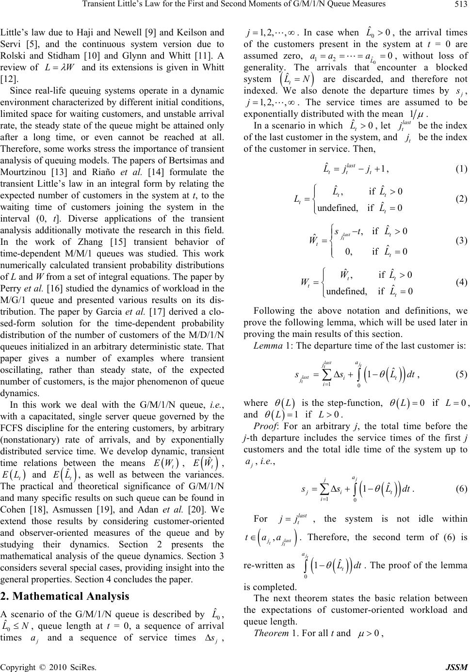

Transient Little’s Law for the First and Second Moments of G/M/1/N Queue Measures513
Little’s law due to Haji and Newell [9] and Keilson and
Servi [5], and the continuous system version due to
Rolski and Stidham [10] and Glynn and Whitt [11]. A
review of LW

 and its extensions is given in Whitt
[12].
Since real-life queuing systems operate in a dynamic
environment characterized by different initial conditions,
limited space for waiting customers, and unstable arrival
rate, the steady state of the queue might be attained only
after a long time, or even cannot be reached at all.
Therefo re, some works str ess the importance of transient
analysis of queuing models. The papers of Bertsimas and
Mourtzinou [13] and Riaño et al. [14] formulate the
transient Little’s law in an integral form by relating the
expected number of customers in the system at t, to the
waiting time of customers joining the system in the
interval (0, t]. Diverse applications of the transient
analysis additionally motivate the research in this field.
In the work of Zhang [15] transient behavior of
time-dependent M/M/1 queues was studied. This work
numerically calculated transient probability distributions
of L and W from a set of integral equations. The paper by
Perry et al. [16] studied the dynamics of workload in the
M/G/1 queue and presented various results on its dis-
tribution. The paper by Garcia et al. [17] derived a clo-
sed-form solution for the time-dependent probability
distribution of the number of customers of the M/D/1/N
queues initialized in an arbitrary deterministic state. That
paper gives a number of examples where transient
oscillating, rather than steady state, of the expected
number of customers, is the major phenomenon of queue
dynamics.
In this work we deal with the G/M/1/N queue, i.e.,
with a capacitated, single server queue governed by the
FCFS discipline for the entering customers, by arbitrary
(nonstationary) rate of arrivals, and by exponentially
distributed service time. We develop dynamic, transient
time relations between the means , 
t
EW


ˆt
EW ,
and , as well as between the variances.
The practical and theoretical significance of G/M/1/N
and many specific results on such queue can be found in
Cohen [18], Asmussen [19], and Adan et al. [20]. We
extend those results by considering customer-oriented
and observer-oriented measures of the queue and by
studying their dynamics. Section 2 presents the
mathematical analysis of the queue dynamics. Section 3
considers several special cases, providing insight into the
general properties. Section 4 concludes the paper.

t
EL

ˆt
EL
2. Mathematical Analysis
A scenario of the G/M/1/N queue is described by 0,
0, queue length at t = 0, a sequence of arrival
times
ˆ
L
ˆ
LN
j
a and a sequence of service times
j
s

,
1, 2,,j

. In case when 0, the arrival times
of the customers present in the system at t = 0 are
assumed zero, 0
ˆ 12 L
ˆ0L
0aaa

, without loss of
generality. The arrivals that encounter a blocked
system


N
ˆt
L are discarded, and therefore not
indexed. We also denote the departure times by
j
s
,
1, 2,,j

. The service times are assumed to be
exponentially distributed with the mean 1

.
In a scenario in which t, let be the index
of the last customer in the system, and be the index
of the customer in service. Then,
ˆ
L
ˆlast
tt
Lj
0
1
t
j
last
t
j
t
j


ˆˆ
,if
ˆ
if 0
t
LL
L


ˆ
,i f
ˆ
if
t
t
L
, (1)
0
t
undefined,
t





ˆ
0,
last
t
j
t
st L
W
t
L (2)
0
0






f
undefine
t





10
last jt
t
st
a
j
i
(3)
ˆˆ
,i
ˆ
d, if
t
t
WL
L

ˆ
1
i
0

0
t


W
la
t
j
(4)
Following the above notation and definitions, we
prove the following lemma, which will be used later in
proving the main results of this section.
Lemma 1: The departure time of the last customer is:

t
s
s  L


dt, (5)
where


L  is the step-function, if

0L  0L

,
and


1L 

if . 0L
Proof: For an arbitrary j, the total time before the
j-th departure includes the service times of the first j
customers and the total idle time of the system up to
j
a, i.e.,
 
ˆ
1

10
j
a
j
ji
it
s
s



t
Ldt  . (6)
For , the system is not idle within
las
t
jj


,last
tt
jj
taa. Therefore, the second term of (6) is
re-written as . The proof of the lemma
is completed.
 
ˆ
1
jt
t
L  

dt
0
0
a

The next theorem states the basic relation between
the expectations of customer-oriented workload and
queue length.
Theorem 1. For all t and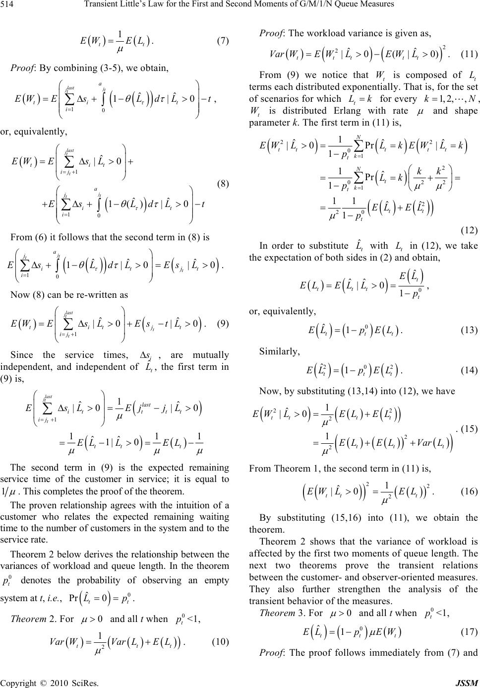

,

Transient Little’s Law for the First and Second Moments of G/M/1/N Queue Measures 514
 
1
t
EW EL

t



t

0
jt
t
. (7)
Proof: By combining (3-5), we obtain,

 
10
ˆˆ
1|0
last j
jt
t
a
ti t
i
EWEsLd Lt





 






,
or, equivalently,


1
10
ˆ
|0
ˆˆ
1() |0
last
jt
t
jt
t
tit
ij
a
j
it
i
EWEs L
Es LdL











 





(8)
From (6) it follows that the second term in (8) is
  
10
ˆˆ ˆ
1|0|
jt
t
t
a
j
it
i
EsLdLEsL





 


.
Now (8) can be re-written as


1
ˆˆ
|0 |0
last
jt
t
t
titj
ij
EWEsLEst L






. (9)
Since the service times, i
s
ˆt
L, are mutually independent, and independent of , the first term in
(9) is,



1
1
ˆˆ
|0 |0
11
ˆˆ
1| 0
last
jt
t
last
itt tt
ij
tt t
EsL EjjL
EL LEL

1





 


 

The second term in (9) is the expected remaining
service time of the customer in service; it is equal to
1

. This completes the proof of the theorem.
The proven relationship agrees with the intuition of a
customer who relates the expected remaining waiting
time to the number of customers in the system and to the
service rate.
Theorem 2 below derives the relationship between the
variances of workload and queue length. In the theorem
denotes the probability of observing an empty
system at t, i.e., .
0
t
p

0
ˆ
Pr 0
tt
Lp
Theorem 2. For 0

 and all t when <1,
0
t
p
   
2
1
tt
Var WVarLEL


Proof: The workload variance is given as,


 
2
2ˆˆ
|0 (|0)
ttttt
VarWEWLE WL. (11)
From (9) we notice that t
W is composed of t
terms each distributed exponentially. That is, for the set
of scenarios for which t
L
Lk

for every 1, 2,,kN

,
t is distributed Erlang with rate W

and shape
parameter k. The first term in (11) is,
  

  
22
01
2
02
1
2
20
1
ˆˆ
|0 Pr|
1
1ˆ
Pr
1
11 ˆˆ
1
N
ttt tt
k
t
N
t
k
t
tt
t
EW LLkEW Lk
p
kk
Lk
p
EL EL
p




 


2
ˆ








(12)
In order to substitute with t in (12), we take
the expectation of both sides in (2) and obtain,
ˆt
L L



0
ˆ
ˆˆ
|0
1
t
ttt
t
EL
ELEL Lp 
,
or, equivalently,





0
ˆ1
tt
ELp EL t . (13)
Similarly,




20
ˆ1
tt
ELp EL2
t
. (14)
Now, by substituting (13,14) into (12), we have




 



22
2
2
2
1
ˆ
|0
1
ttt t
tt
EW LELEL
EL ELVarL


 

t
. (15)
From Theorem 1, the second term in (11) is,





22
2
1
ˆ
|0
tt t
EW LEL



. (16)
By substituting (15,16) into (11), we obtain the
theorem.
Theorem 2 shows that the variance of workload is
affected by the first two moments of queue length. The
next two theorems prove the transient relations
between the customer- and observer-oriented measures.
They also further strengthen the analysis of the
transient behavior of the measures.
Theorem 3. For 0

 and all t when <1,
0
t
p





0
ˆ1
tt
ELp EW   t (17)
t
. (10) Proof: The proof follows immediately from (7) and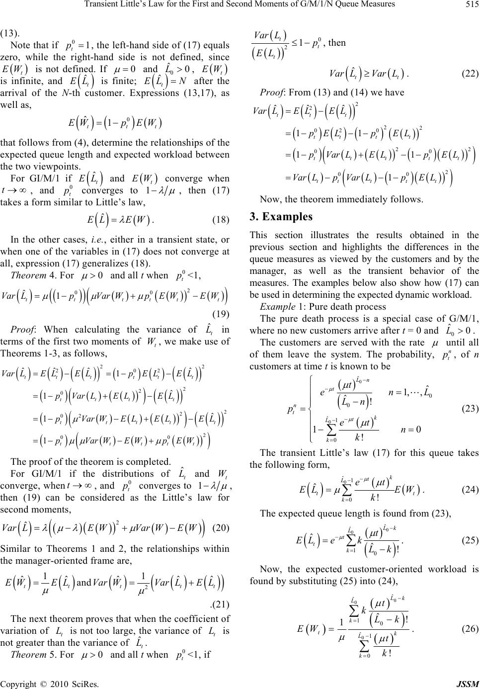

Transient Little’s Law for the First and Second Moments of G/M/1/N Queue Measures515
(13).
Note that if , the left-hand side of (17) equals
zero, while the right-hand side is not defined, since
is not defined. If
01
t
p

t
EW 0


and ,
0
ˆ0L


t
EW
is infinite, and is finite; after the
arrival of the N-th customer. Expressions (13,17), as
well as,

ˆt
EL
 
tN
ˆ
EL



0
ˆ1
tt
EWpEWt
that follows from (4), determine the relationships of the
expected queue length and expected workload between
the two viewpoints.
For GI/M/1 if and converge when
, and converges to

ˆt
EL

t
EW
t 0
t
p1

 , then (17)
takes a form similar to Little’s law,


ˆ
EL EW  . (18)
In the other cases, i.e., either in a transient state, or
when one of the variables in (17) does not converge at
all, expression (17) generalizes (18).
Theorem 4. For 0

 and all t when <1,
0
t
p



 



2
00
ˆ1
ttttt
VarLpVarWp EWEW  
t
(19)
Proof: When calculating the variance of
te
ˆ in
t
L
rms of the f irst two moments of t
W, we make use of
Theorems 1-3, as follows,
 


 



 





 


 

 


0 2
2
2
0
2
2
02
2
00
ˆˆ ˆˆ
1
ˆ
1
ˆ
1
1
tt ttt t
ttt t
tttt
ttttt
VarLELELp ELEL
pVarL ELEL
pVarWELEL EL
pVarWEWpEW

 
 


 
2
22
t
The proof of the theorems completed.
For GI/M/1 if the disibutions of and
co
i
tr ˆt L
s tot
W
nverge, whent, and 0 p converge
t 1



,
forth
Similar to Theorems 1 and 2, the relationships w
the manager-oriented frame are,
en (19) can be considered as the Littl law
second moments,

   

2
ˆ
VarLE WVar WE W    (20)
e’s
ithin
 
1
ˆˆ
tt
EW EL

and
  

2
1
ˆˆˆ
t
Var W
tt
Var LE L


.(21
The next theorem proves that when the coefficient
variation of is not too large, the variance of
no
)
of
L is
t t
t greater than the variance of ˆt L.
Theorem 5. For 0
L

 and all t when 0
t
p<1, if


 
0
21
tt
p
Var L

, then
t
EL



ˆtt
Var L.Var L (22)
Proof: From (13) and (14) we have
 


ˆˆ ˆ
tt t
r LE LE L

 

  

 

 




2
2
22
02 0
22
00
2
00
11
11
1
tt t t
ttt tt
tttt t
Va
pELp EL
pVarLELpEL
Var LpVar LpEL
 
 
 
Now, the theorem immediately follows.
3.
ustrates the results obtained in the
and highlights the differences in the
,
wt = 0 and .
Examples
This section ill
previous section
queue measures as viewed by the customers and by the
manager, as well as the transient behavior of the
measures. The examples below also show how (17) can
be used in determining the expected dynamic workload.
Example 1: Pure death process
The pure death process is a special case of G/M/1
here no new customers arrive after 0
The customers are served with the rate
ˆ0
L

until all
of them leave the system. The probability, n
n
t
p, of
customers at time t is known to be



0
ˆ
ˆ
Ln
tt
en






0
0
0
ˆ1
0
ˆ
1, ,
!
10
!
n
tk
t
L
k
L
Ln
p
et n
k














(23)
The transient Little’s law (17) for this queue takes
the following form,



0
ˆ1
ˆk
t
L
t
et
EL





0!t k
EW
k


. (24)
The expected queue length is found from (23),



0
0
ˆ
ˆˆ
10
ˆ!
L
k
L
t
t
t
EL ek



.
kLk

 (25)
Now, the expected customer-ori
found by substituting (25) into (24), ented workload is


0
0ˆ
ˆ


0
10
ˆ1
0
ˆ!
1
!
L
k
Lt
k



k
tk
L
k
Lk
EW t
k







. (26)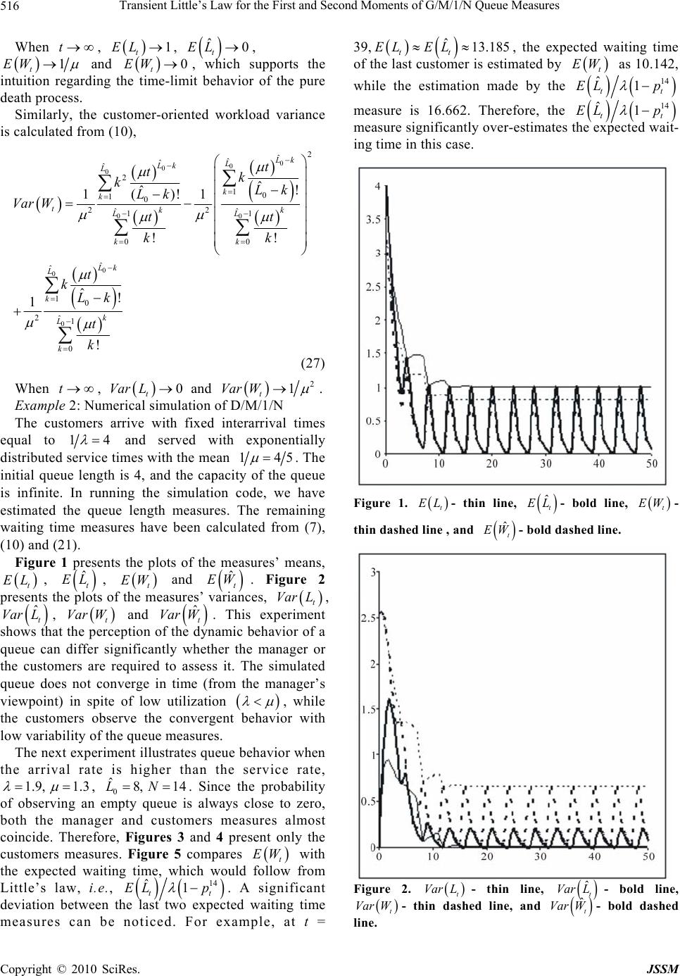

Transient Little’s Law for the First and Second Moments of G/M/1/N Queue Measures 516
When t , ,

1
t
EL ,

ˆ0
t
EL 

1
t
EW


intuition regard
and supports the
i
death process.
Similarly, the customer-oriented workload variance
is calculated from (10),

t
EW 
ng the time-lim
0, which
it behavior of the pure









0
0
0
2
ˆ
ˆ
ˆ2
10
ˆ!
ˆ
()! 11
Lk
L
L
k
t
tk
kLk
Lk
Var W











0
0
0
0
ˆ
10
0
ˆ
ˆ
10
2ˆ1
0
!!
ˆ!
1
!
Lk
k
k
Lk
L
k
k
L
k
kk
t
kLk
t
k

















(27)
When and
00
22
ˆˆ
11
0
tkk
LL
k
tt







t,

0
t
Var L

2
1
t
Var W

.
Example on of D/M/1/N
The customers arrive with fixed interarrival times
equal to
2: Numerical simulati
14


ic and served with exponentially distributed serve times with the mean 145

. The
eue initial queue length is 4, and the capacity of the qu
is . In rning the sim code, we hav
estning
w). asures’ m
infiniteunulatione
imated the queue length measures. The remai
aiting time measures have been calculated from (7),
(10) and (21
Figure 1 presents the plots of the meeans,

t
EL ,

ˆt
EL ,

t
EW and

ˆt
EW . Figure 2
presents the plots of the measures’ variances,


t
Var L,

ˆt
Var L,

t
Var W and

ˆt
Var W. This experiment
shows that the perception of the dynamic behavior of a
queue can differ significant
t converge in
ly whether th
(from the
e manager or

the
queue does no
customers are required to assess it. The simulated
time manager’s
viewpoint) in spite of low utilization


 
omve theent behavior with
low variability of the queue measures.
The next experiment illustrates queue behavior when
the arrival rate is higher than the service rate,
1.9, 1.3
, while
the custers obser converg

 , 0
ˆ8, 14
LN. Since the probability
of observing an empty queue is alwayso zero,
both the manager and customers measures almost
coincide. Therefore, Figures 3 and 4
close t
present only the
cu
Little’s law, i.
stomers measures. Figure 5 compares

t
EW with
the expected waiting time, which would follow from
e.,



14
t
p. A significant
deviation between the last two expected waiting time
measures can be noticed. For example, at t =
39,

ˆ1
t
EL 


ˆ13.185
tt
EL EL, the expected waiting time
of the last customer is estimated by

t
EW 0.142,
while the estimation made b

e

as 1
y th


14
ˆ1
tt
p  
measure is 16.662. Therefore, the

EL


14
ˆ1
tt
EL p  
measure significantly over-estimates the expected wait-
ing
time in this case.
gure 1.


t
EL - thin line,

ˆt
ELFi - bold li


t
EWne, -
thin dashed line , and


ˆt
EW - bold dashed line.
gure 2.


t
Var L- thin line, - bold line,

ˆt
Var L


t
W- thin dashed line
Fi
Var


ˆt
W- bo, and Var ld dashed
line.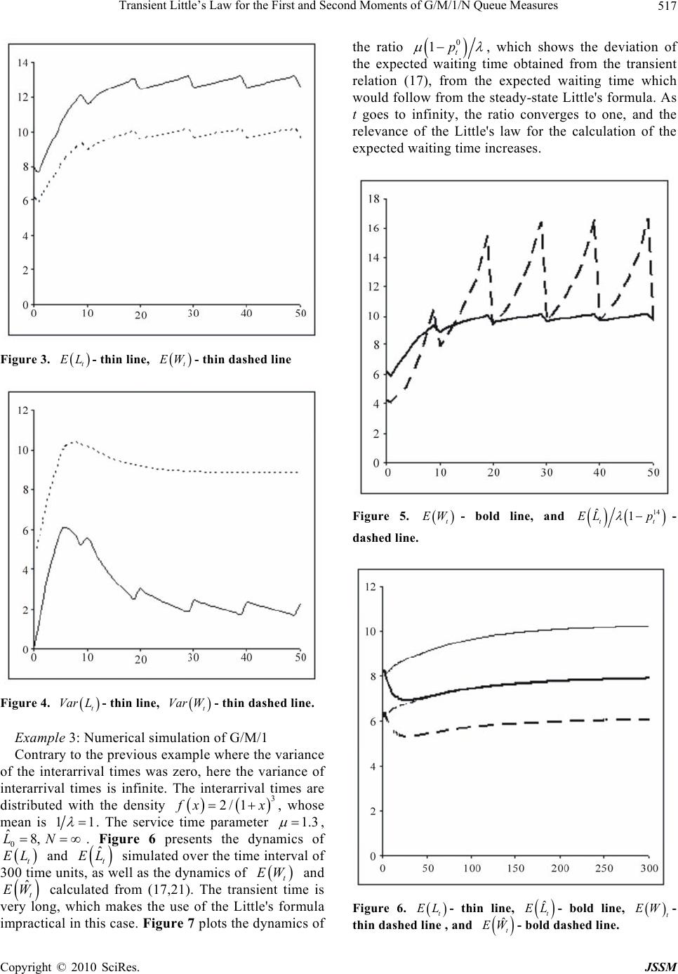

Transient Little’s Law for the First and Second Moments of G/M/1/N Queue Measures517
Figure 3.


t
EL - thin line,


t
EW - thin dashed line
Figure 4. - thin line,

t
Var L


t
Var W- thin dashed line.
e 3: Nmulati
Contr ary to the previous example where the variance
f the interarrival times was zero, here the variance of
interarrival times is infinite. The interarrival times are
distributed with the density
Exampl umerical sion of G/M/1
o
 
3
2/ 1
f
xx, whose
mean is 11

. The service time parameter 1.3


,
ics of
erval of
0
ˆ8,LN

t
EL and
300 time unit
 . Figure 6 p
simula
l as th
resents the dynam
ted over the time int
e dynamics of

ˆt
EL
s, as wel


t and
ent time is
mula
EW
The transi
se of the Little's for

ˆt
EW calculated
very long, whfrom (17,21). kes the u
impractical in this case. Figure 7 plots the dynamics of
the ratio
ich ma


0
1t p

 
the expected waiting tim
m
ow from the st
infinity, th
he Littl
waiting time
, which shows the deviation of
e obtained from the transient
relation (17), frothe expected waiting time which
would folleady-state Little's formula. As
t goes toe ratio converges to one, and the
relevance of te's law for the calculation of the
expected increases.
Figure 5.


t
EW - bold line, and




14
ˆtt
EL p  -
line.
1
dashed
- thin line,


ˆt
EL


t
EL - bold line,


t
EW Figure 6.-
thin dasheand d line ,


ˆt
EW - bold dashed line.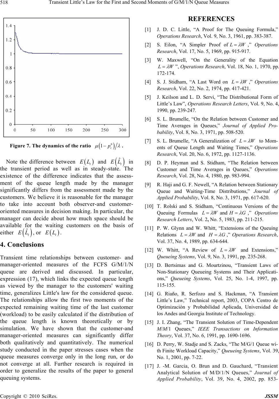

Transient Little’s Law for the First and Second Moments of G/M/1/N Queue Measures 518
Figure 7. The dynamics of the ratio


0
1t p

 .
Note the difference between and

t
EL


ˆt
EL
tate. Th
asse
manag
ade by the
the manager
custom
ticular, the
space should
the basis of
in
t period as well eady-se
istence of the difference ind that thess-
ment of the queue length mde by the er
significantly differs from the assnt m
customers. We believe it is ree for
to take into account both r-and er-
oriented measures in decision mIn par
manager can decide about how be
available for the waiting custo
either , or
4. Conclusions
Transient time relationships between customer- and
manager-oriented measures of the FCFS G/M/1/N
queue are derived and discussed. In particular,
expression (17), which links the expected queue length
as viewed by the manager to the customers' waiting
time, generalizes Little's law for the considered queue.
The relationships allow the first two moments of the
expected remaining waiting time of the last customer
lated
is kn or by
simulation. We have shown that the customer-and
manager-oriented measures can significantly differ
both qualitatively and quantitatively. The numerical
study conducted in the paper stresses cases when the
queue measures converge only in the long run, or do
not converge at all. Further research is required in
order to generalize the results of the paper to general
queuing systems.
REFERENCES
[1] J. D. C. Little, “A Proof for The Queuing Formula,”
Operations Research, Vol. 9, No. 3, 1961, pp. 383-387.
[2] S. Eilon, “A Simpler Proof o
th
exe transienas in st
icates
aessme
asonabl
observe
aking.
much
mers on

ˆt
EL

t
EL .
(workload) to be easily calcuif the distribution of
the queue length own theoretically
f
L
W

,” Operations
Research, Vol. 17, No. 5, 1969, pp. 915-917.
[3] W. Maxwell, “On the Generality of the Equation
L
W


”, Operations Research, Vol. 18, No. 1, 1970, pp.
172-174.
[4] S. J. Stidham, “A Last Word on
L
W

,” Operations
Research, Vol. 22, No. 2, 1974, pp. 417-421.
[5] J. Keilson and L. D. Servi, “The Distributional Form of
Little’s Law”, Operations Research Letters, Vol. 9, No. 4,
1990, pp. 239-247.
[6] S. L. Brumelle, “On the Relation between Customer and
Time Averages in Queues,” Journal of Applied Pro-
bability, Vol. 8, No. 3, 1971, pp. 508-520.
[7] S. L. Brumelle, “A Generalization of
L
W

 to Mom
imes,” Operations
Research, Vol. 20, No. 6, 1972, pp. 1127-1136.
[8] , “Then betw
-
ents of Queue Length and Waiting T
D. P. Heyman and S. Stidham Relatioeen
Customer and Time Averages in Queues,” Operations
Research, Vol. 28, No. 4, 1980, pp. 983-994.
[9] R. Haji and G. F. Newell, “A Relation between Stationary
Queue and Waiting-Time Distributions,” Journal of
Applied Probability, Vol. 8, No. 3, 1971, pp. 617-620.
[10] T. Rolski and S. Stidham, “Continuous Versions of the
Queuing Formulas
L
W


and HG

,” Operations
Research Letters, Vol. 2, No. 5, 1983, pp. 211-215.
[11] P. W. Glynn and W. Whitt, “Extensions of the Queuing
Re lations
L
W


and HG

,” Operations Research,
989, pp. 634-644. Vol. 37, No. 4, 1
[12] W. Whitt, “A Review of
L
W

 and Extensions,”
bility, Vol. 39, No. 4, 2002, pp. 853-
Queueing Systems, Vol. 9, No. 3, 1991, pp. 235-268.
[13] D. Bertsimas and G. Mourtzinou, “Transient Laws of
Non-Stationary Queueing Systems and Their Applicati-
ons,” Queueing Systems, Vol. 25, No. 1-4, 1997, pp.
115-155.
[14] G. Riaño, R. Serfozo and S. Hackman, “A Transient
Little’s Law,” Technical report, 2003, COPA Centro de
Optimización y Probabilidad Aplicada, Universidad de
los Andes and Georgia Institute of Technology.
[15] J. I. Zhang, “The Transient Solution of Time-Dependent
M/M/1 Queues,” IEEE Transactions on Information
Theory, Vol. 37, No. 6, 1991, pp. 1690-1696.
[16] D. Perry, W. St adje and S. Zack s, “The M/G/1 Que ue wi-
th Finite Workload Capacity,” Queueing Systems, Vol. 39,
No. 1, 2001, pp. 7-22.
[17] J. -M. Garcia, O. Brun and D. Gauchard, “Transient
Analytical Solution of M/D/1/N Queues,” Journal of
Applied Proba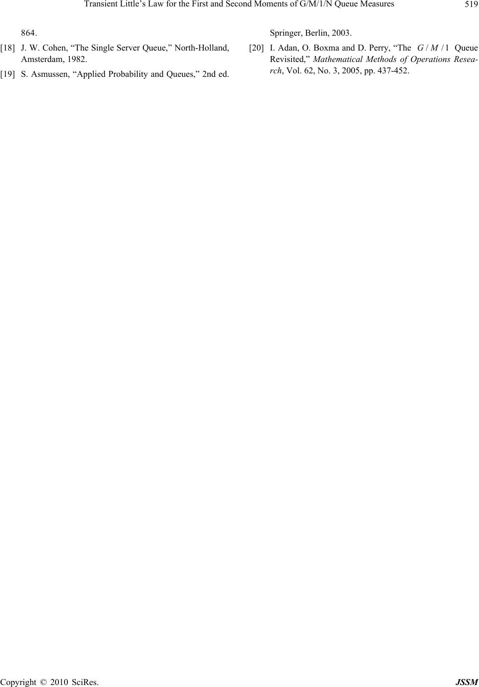

Transient Little’s Law for the First and Second Moments of G/M/1/N Queue Measures 519
864.
The Queue
Springer, Berlin, 2003.
[20] I. Adan, O. Boxma and D. Perry, “//1GM [18] J. W. Cohen, “The Single Server Queue,” North-Holland,
Amsterdam, 1982. Revisited,” Mathematical Methods of Operations Resea-
rch, Vol. 62, No. 3, 2005, pp. 437-452.
[19] S. Asmussen, “Applied Probability and Queues,” 2nd ed.