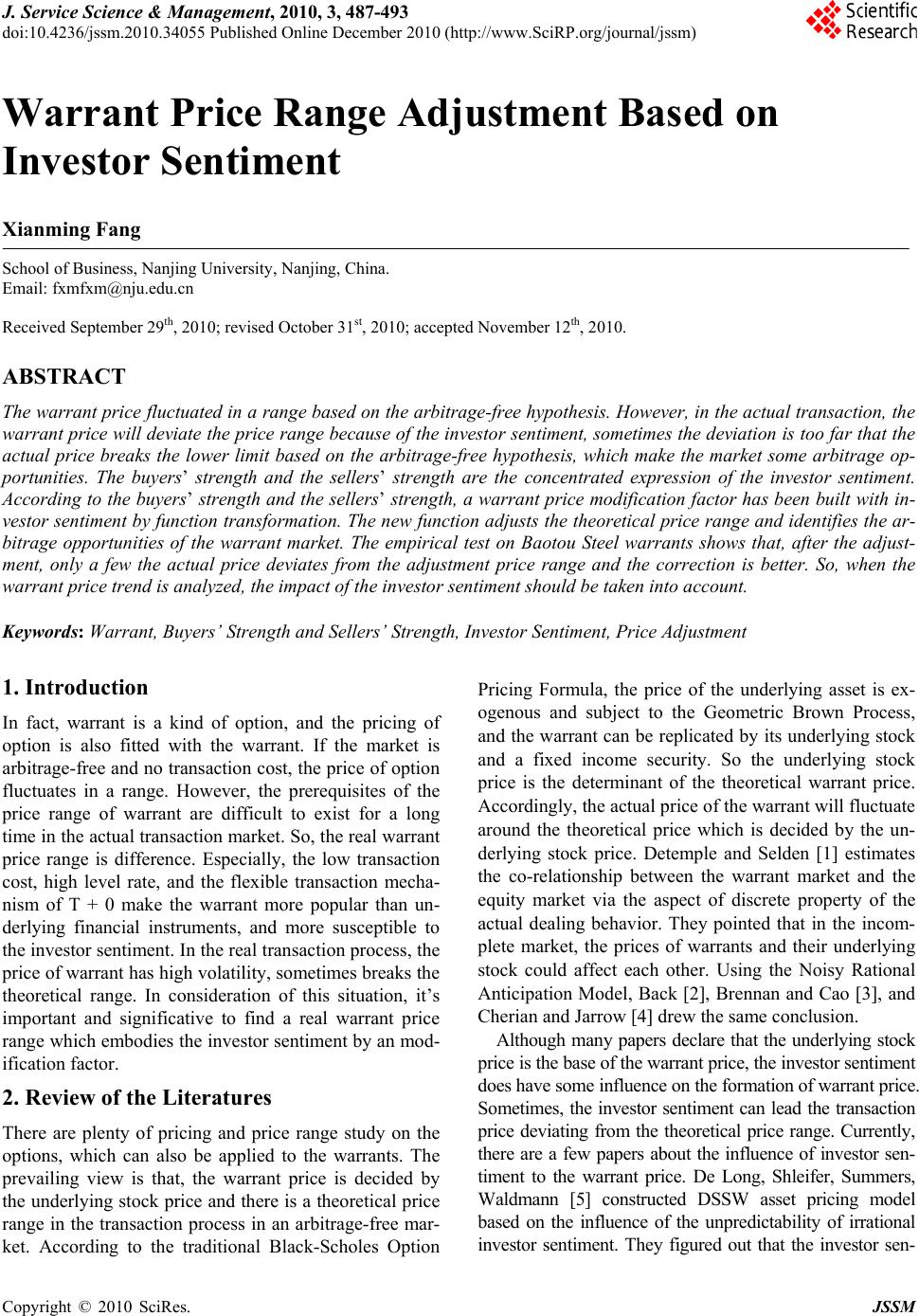J. Service Science & Management, 2010, 3, 487-493
doi:10.4236/jssm.2010.34055 Published Online December 2010 (http://www.SciRP.org/journal/jssm)
487
Warrant Price Range Adjustment Based on
Investor Sentiment
Xianming Fang
School of Business, Nanjing University, Nanjing, China.
Received September 29th, 2010; revised October 31st, 2010; accepted November 12th, 2010.
ABSTRACT
The warrant price fluctuated in a range based on the arbitrage-free hypothesis. However, in the actual transaction, the
warrant price will deviate the p rice range because of the investo r sentiment, sometimes the deviation is too far that the
actual price breaks the lower limit based on the arbitrage-free hypothesis, which make the market some arbitrage op-
portunities. The buyers’ strength and the sellers’ strength are the concentrated expression of the investor sentiment.
According to the buyers’ strength and the sellers’ strength, a warrant price modification factor has been built with in -
vestor sentiment by func tion transformation. The new function adjusts the theoretica l price range and identifies the ar-
bitrage opportunities of the warrant market. The empirical test on Baotou Steel warrants shows that, after the adjust-
ment, only a few the actual price deviates from the adjustment price range and the correction is better. So, when the
warrant price trend is analyzed, the impact of th e investor sentiment should be taken into ac count.
Keywords: Warrant, Buyers’ Strength and Sellers’ Strength, Investor Sentiment, Price Adjustment
1. Introduction
In fact, warrant is a kind of option, and the pricing of
option is also fitted with the warrant. If the market is
arbitrage-free and no transaction cost, the price of option
fluctuates in a range. However, the prerequisites of the
price range of warrant are difficult to exist for a long
time in the actual transaction market. So, the real warrant
price range is difference. Especially, the low transaction
cost, high level rate, and the flexible transaction mecha-
nism of T + 0 make the warrant more popular than un-
derlying financial instruments, and more susceptible to
the investor sentiment. In th e real transaction process, the
price of warrant has high volatility, sometimes break s the
theoretical range. In consideration of this situation, it’s
important and significative to find a real warrant price
range which embodies the investor sentiment by an mod-
ification factor.
2. Review of the Literatures
There are plenty of pricing and price range study on the
options, which can also be applied to the warrants. The
prevailing view is that, the warrant price is decided by
the underlying stock price and there is a theoretical price
range in the transaction process in an arbitrage-free mar-
ket. According to the traditional Black-Scholes Option
Pricing Formula, the price of the underlying asset is ex-
ogenous and subject to the Geometric Brown Process,
and the warrant can be replicated by its underlying stock
and a fixed income security. So the underlying stock
price is the determinant of the theoretical warrant price.
Accordingly, the actual pr ice of th e warrant will flu ctuate
around the theoretical price which is decided by the un-
derlying stock price. Detemple and Selden [1] estimates
the co-relationship between the warrant market and the
equity market via the aspect of discrete property of the
actual dealing behavior. They pointed that in the incom-
plete market, the prices of warrants and their underlying
stock could affect each other. Using the Noisy Rational
Anticipation Model, Back [2], Brennan and Cao [3], and
Cherian and Jarrow [4] drew the same conclusion.
Although many papers declare that the underlying stock
price is the base of the warrant price, the investor sentiment
does have some influence on the formation of warrant price.
Sometimes, the investor sentiment can lead the transaction
price deviating from the theoretical price range. Currently,
there are a few papers about the influence of investor sen-
timent to the warrant price. De Long, Shleifer, Summers,
Waldmann [5] constructed DSSW asset pricing model
based on the influence of the unpredictability of irrational
investor sentiment. They figured out that the investor sen-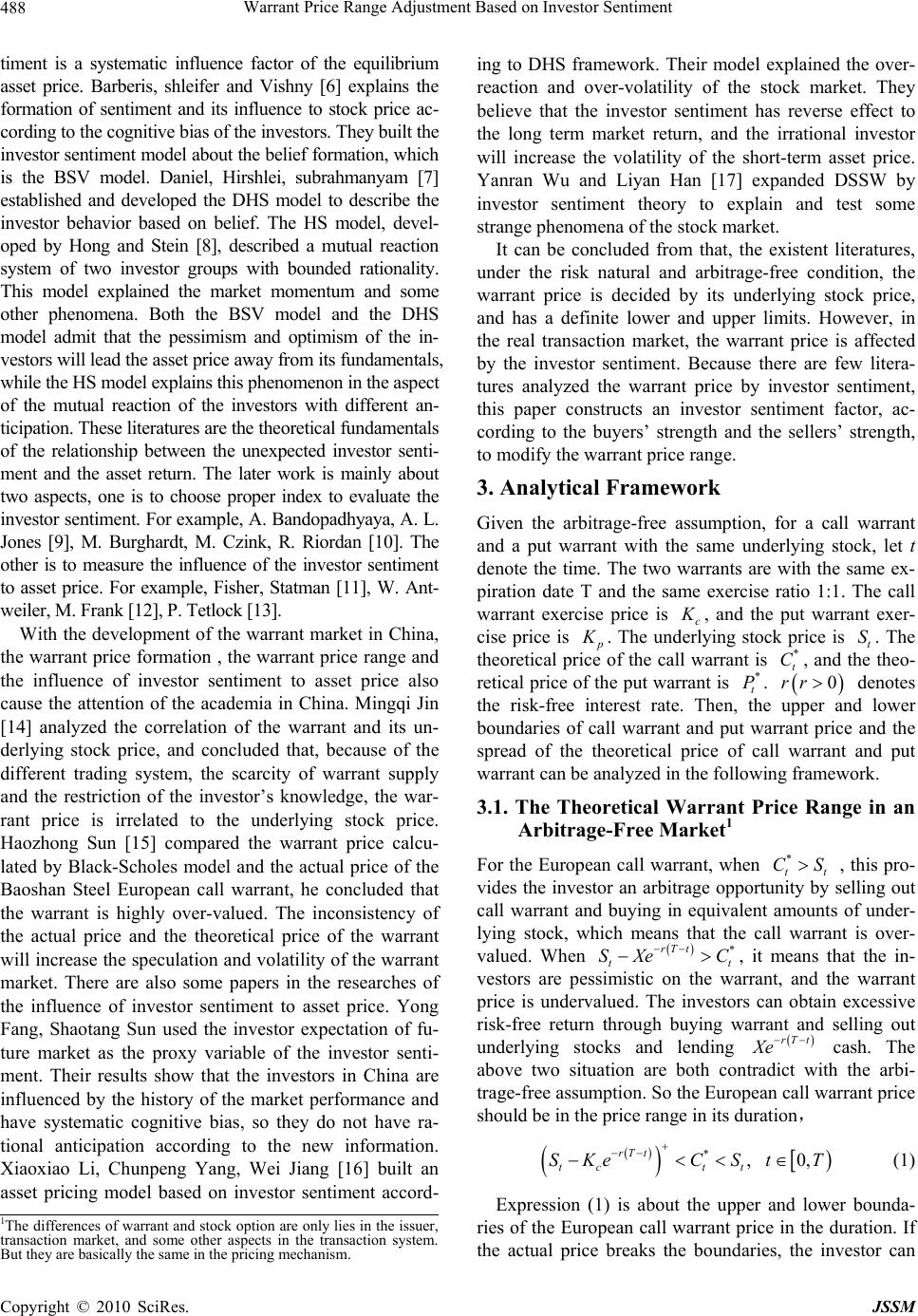

Warrant Price Range Adjustment Based on Investor Sentiment 488
timent is a systematic influence factor of the equilibrium
asset price. Barberis, shleifer and Vishny [6] explains the
formation of sentiment and its influence to stock price ac-
cording to the cognitive bias of the investors. They built the
investor sentiment model about the belief formation, which
is the BSV model. Daniel, Hirshlei, subrahmanyam [7]
established and developed the DHS model to describe the
investor behavior based on belief. The HS model, devel-
oped by Hong and Stein [8], described a mutual reaction
system of two investor groups with bounded rationality.
This model explained the market momentum and some
other phenomena. Both the BSV model and the DHS
model admit that the pessimism and optimism of the in-
vestors will lead the asset price away from its fundamentals,
while the HS model explains this phenomenon in the aspect
of the mutual reaction of the investors with different an-
ticipation. These literatures are the theoretical fundam e ntals
of the relationship between the unexpected investor senti-
ment and the asset return. The later work is mainly about
two aspects, one is to choose proper index to evaluate the
investor sentiment. For example, A. Bandopadhyaya, A. L.
Jones [9], M. Burghardt, M. Czink, R. Riordan [10]. The
other is to measure the influence of the investor sentiment
to asset price. For example, Fisher, Statman [11], W. Ant-
weiler, M. Frank [12], P. Tetlock [13].
With the development of the warrant market in China,
the warrant price formation , the warrant price range and
the influence of investor sentiment to asset price also
cause the attention of the academia in China. Mingqi Jin
[14] analyzed the correlation of the warrant and its un-
derlying stock price, and concluded that, because of the
different trading system, the scarcity of warrant supply
and the restriction of the investor’s knowledge, the war-
rant price is irrelated to the underlying stock price.
Haozhong Sun [15] compared the warrant price calcu-
lated by Black-Scholes model and the actual price of the
Baoshan Steel European call warrant, he concluded that
the warrant is highly over-valued. The inconsistency of
the actual price and the theoretical price of the warrant
will increase the speculation an d volatility of the warrant
market. There are also some papers in the researches of
the influence of investor sentiment to asset price. Yong
Fang, Shaotang Sun used the investor expectation of fu-
ture market as the proxy variable of the investor senti-
ment. Their results show that the investors in China are
influenced by the history of the market performance and
have systematic cognitive bias, so they do not have ra-
tional anticipation according to the new information.
Xiaoxiao Li, Chunpeng Yang, Wei Jiang [16] built an
asset pricing model based on investor sentiment accord-
ing to DHS framework. Their model explained the over-
reaction and over-volatility of the stock market. They
believe that the investor sentiment has reverse effect to
the long term market return, and the irrational investor
will increase the volatility of the short-term asset price.
Yanran Wu and Liyan Han [17] expanded DSSW by
investor sentiment theory to explain and test some
strange phenomena of the stock market.
It can be concluded from that, the existent literatures,
under the risk natural and arbitrage-free condition, the
warrant price is decided by its underlying stock price,
and has a definite lower and upper limits. However, in
the real transaction market, the warrant price is affected
by the investor sentiment. Because there are few litera-
tures analyzed the warrant price by investor sentiment,
this paper constructs an investor sentiment factor, ac-
cording to the buyers’ strength and the sellers’ strength,
to modify the warrant price range.
3. Analytical Framework
Given the arbitrage-free assumption, for a call warrant
and a put warrant with the same underlying stock, let t
denote the time. The two warrants are with the same ex-
piration date T and the same exercise ratio 1:1. The call
warrant exercise price is c
K
, and the put warrant exer-
cise price is
p
K
. The underlying stock price is t. The
theoretical price of the call warrant is , and the theo-
retical price of the put warrant is . denotes
the risk-free interest rate. Then, the upper and lower
boundaries of call warrant and put warrant price and the
spread of the theoretical price of call warrant and put
warrant can be analyzed in the following framework.
S

*
t
C
rr
*
t
P

0
3.1. The Theoretical Warrant Price Range in an
Arbitrage-Free Market1
For the European call warrant, when , this pro-
vides the investor an arbitrage opportunity by selling out
call warrant and buying in equivalent amounts of under-
lying stock, which means that the call warrant is over-
valued. When t
, it means that the in-
vestors are pessimistic on the warrant, and the warrant
price is undervalued. The investors can obtain excessive
risk-free return through buying warrant and selling out
underlying stocks and lending cash. The
above two situation are both contradict with the arbi-
trage-free assumption. So the European call warrant price
should be in the price range in its duration，
*
tt
CS

rT t
 *
rT t
t
SXeC


Xe





*, 0,
rT t
tc tt
SKeC StT


 (1)
Expression (1) is about the upper and lower bounda-
ries of the European call warrant price in the duration. If
the actual price breaks the boundaries, the investor can
1The differences of warrant and stock option are only lies in the issuer,
transaction market, and some other aspects in the transaction system.
But the
y
are basicall
y
the same in the
p
ricin
g
mechanism.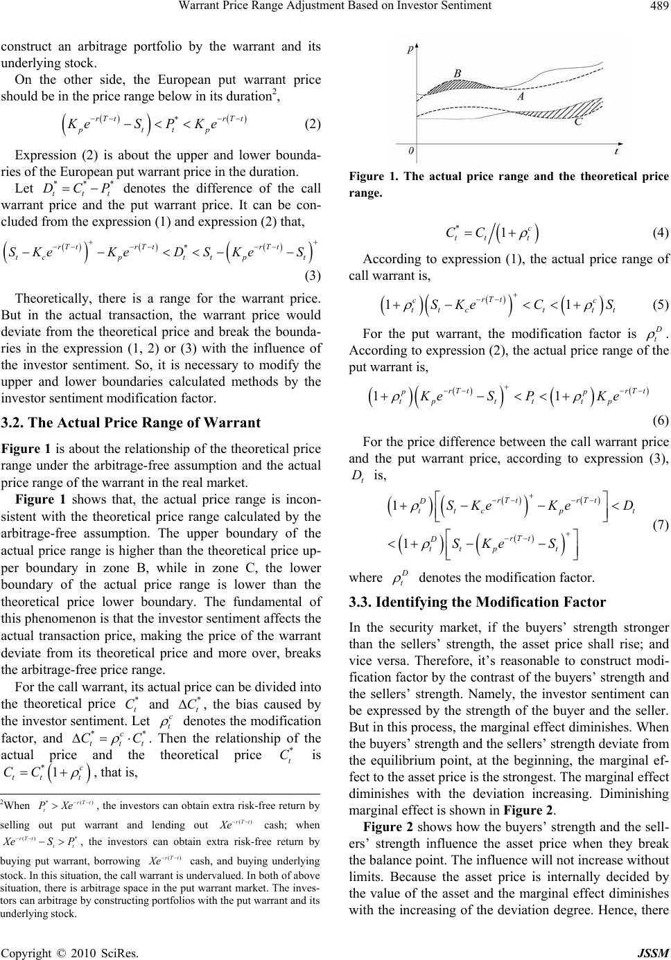

Warrant Price Range Adjustment Based on Investor Sentiment489
*
construct an arbitrage portfolio by the warrant and its
underlying stock.
On the other side, the European put warrant price
should be in the price range below in its duration2,


 *
rT trT t
pttp
KeSP Ke
 
 (2)
Expression (2) is about the upper and lower bounda-
ries of the European put warrant price in the duration.
Let t
denotes the difference of the call
warrant price and the put warrant price. It can be con-
cluded from the expression (1) and expression (2) that,
**
tt
DCP



 


*
rT trTtrT t
tcptt pt
SKeKeD SKeS

 

(3)
Theoretically, there is a range for the warrant
B
rant
al price
e is incon-
si
l price can be divided into
th
price.
ut in the actual transaction, the warrant price would
deviate from the theoretical price and break the bounda-
ries in the expression (1, 2) or (3) with the influence of
the investor sentiment. So, it is necessary to modify the
upper and lower boundaries calculated methods by the
investor senti m ent modification fac t or .
3.2. The Actual Price Range of War
Figure 1 is about the relationship of the theo retic
range under the arbitrage-free assumption and the actual
price range of the warrant in the real market.
Figure 1 shows that, the actual price rang
stent with the theoretical price range calculated by the
arbitrage-free assumption. The upper boundary of the
actual price range is higher than the theoretical price up-
per boundary in zone B, while in zone C, the lower
boundary of the actual price range is lower than the
theoretical price lower boundary. The fundamental of
this phenomenon is that the in vestor sentimen t affects the
actual transaction price, making the price of the warrant
deviate from its theoretical price and more over, breaks
the arbitrage-free price range.
For the call warrant, its actua
e theoretical price *
t
C and *
t
C, the bias caused by
the investor sentimentet c
t
. L

otes the modification
factor, and **c
ttt
CC  . the relationship of the
actual pric theoretical price *
t
C is

*1c
tt t
CC
den
enTh
e and the

, that is,
Figure 1. The actual price range and the theoretical price
range.


*1c
tt t
CC

 (4)
According to expression (1), th
ca e actual price range of ll warrant is,



 
11
rT t
ttct t
SKe CS 


 
cc
t
(5)
For the put warrant, the modification factor is
D
t

.
According to expr ession (2), the actual price range of the
put warrant is,



 

11
rT trT t
tpt ttp
KeS PKe 

pp




6)
For the price difference between the call warrant p
an
(
rice
d the put warrant price, according to expression (3),
t
D is,








1
1
rT trT t
D
ttc p
rT t
D
tt pt
SKeKeD
SKe S



 



t





 



(7)
where
D
t

denotes the modification factor.
ent
stronger
ength and the sell-
er
3.3. Idifying the Modification Factor
In the security market, if the buyers’ strength
than the sellers’ strength, the asset price shall rise; and
vice versa. Therefore, it’s reasonable to construct modi-
fication factor by the contrast of the buyers’ strength and
the sellers’ strength. Namely, the investor sentiment can
be expressed by the strength of the buyer and the seller.
But in this process, the marginal effect diminishes. When
the buyers’ strength and the sellers’ strength deviate from
the equilibrium point, at the beginning, the marginal ef-
fect to the asset price is the strongest. The marginal effect
diminishes with the deviation increasing. Diminishing
marginal effect is shown in Figure 2.
Figure 2 shows how the buyers’ str
s’ strength influence the asset price when they break
the balance point. The influence will not increase without
limits. Because the asset price is internally decided by
the value of the asset and the marginal effect diminishes
with the increasing of the deviation degree. Hence, there
2When )
, the investors can obtain extra risk-free return by
*(rTt
t
PXe


selling out put warrant and lending out cash; when
, the investors can obtain extra risk-free return by
buying put warrant, borrowing cash, and buying underlying
stock. In this situation, the call warrant is undervalued. In both of above
situation, there is arbitrage space in the put warrant market. The inves-
tors can arbitrage by constructing portfolios with the put warrant and its
underlying stock.
()rTt
Xe
() *t
tt
S P
rT
Xe
()rT t
Xe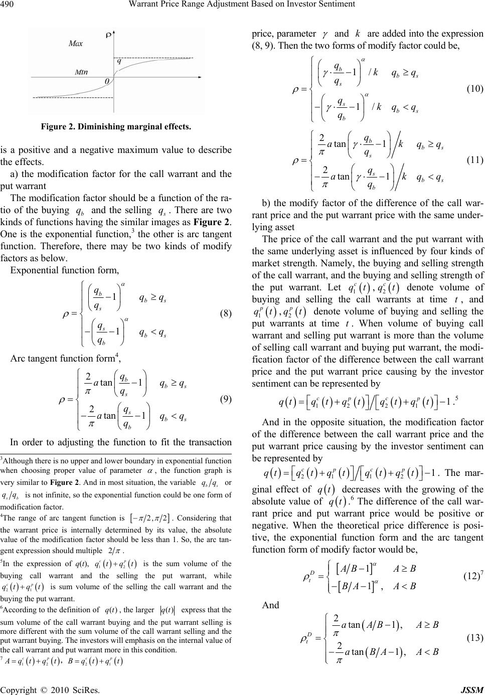

Warrant Price Range Adjustment Based on Investor Sentiment 490
Figure 2. Diminishing marginal effects.
a positive and a negative maximum value to describe
dification factor for the call warrant and the
pu ication factor should be a functio n of the ra-
tio
is
the effects.
a) the mo
t warrant
The modif
of the buying b
q and the selling
s
q. There are two
kinds of functions ving the similar imes as Figure 2.
One is the exponential function,3 the other is arc tangent
function. Therefore, there may be two kinds of modify
factors as below.
Exponential fun
ha ag
ction form,
1
1
bbs
s
sbs
b
qqq
q
qqq
q









 



(8)
Arc tangent function form4,
2q

tan 1
2tan 1
bbs
s
sbs
b
aq q
q
q
aqq
q





 





(9)
In order to adjusting the function to fit the transaction
price, parameter

and k are added into the expression
(8, 9). Then the two forms f modify factor could be, o
1/
1/
bbs
s
sbs
b
qkqq
q
qkq q
q














 



(10)
2tan 1
2tan1
bbs
s
sbs
b
q
ak
q
q
ak
q






qq
qq



 



 



(11)
b) the modify factor of the difference of the call war-
ra
of the call warrant and the put warrant with
th
nt price and the put warrant price with the same under-
lying asset
The price
e same underlying asset is influenced by four kinds of
market strength. Namely, the buying and selling strength
of the call warrant, and th e buying and selling str ength of
the put warrant. Let


1
c
qt,

2
c
qt denote volume of
buying and selling the wts at time t, and call arran


1
p
qt,


2
p
qt denote volume of buying and selling the
rat time t. When volume of buying call
warrant and selling putwarrant is more than the volume
of selling call warrant and buying put warrant, the modi-
fication factor of the difference between the call warrant
price and the put warrant price causing by the investor
sentiment can be represented by
put warants






12 211
cp c
qtqt qtqp t qt

 



 .5
And in the opposite situation, the modification factor
of the difference between the call warrant price and the
put warrant price causing by the investor sentiment can
be represented by




3Although there is no upper and lower boundary in exponential function
when choosing proper value of parameter

, the function graphis
very similar to Figure 2. And in most situation, the variable bs
qq or
s
b
qq is not infinite, so the exponential function could be one form o
f
modification factor.
4The range of arc tangent function is


2, 2  . Considering that
the warrant price is internally determined by its value, the absolute
value of the modification factor should be less than 1. So, the arc tan-
gent expression should multiple 2

.
5In the expression of q(t),



12
cp
qt qt is the sum volume of the
buying call warrant and the selling the put warrant, while
is sum volume of the selling the call warrantand the
buying the put warrant.
 
21
cp
qt qt
6According to the definition of , the larger ()qt ()qt express that the
sum volume of the call warrant buying and the put warrant selling is
more different with the sum volume of the call warrant selling and the
p
ut warrant buying. The investors will empha sis on the in ternal value o
f
the call warrant and put warrant more in this condition.
7
  
12 21
cp cp
A
qt qtBqt qt ，


21
c
qtqtq1 21
p cp
tq tqt

 



 . The mar-
ginal effect of


qt decreases with the growing of the
absolute value of


t.6 The difference of the call war-
rant price and purant price would be positive or
negative. When the theoretical price difference is posi-
tive, the exponential function form and the arc tangent
function form of modify factor would be,
q
t war


1,
D
t
1
A
BAB


BA A B










(12)
7
And


2tan1 ,
2tan1 ,
D
t
aAB A
aBA A








B
B




(13)

Warrant Price Range Adjustment Based on Investor Sentiment491
When the price difference of call warrant price and put
warrant price is negative, the plus signs in fr
modify factor expressions above should be r
the minus signs. At the same time, the minus signs
sh
h as Bao Steel JTB1,
B1,
W, etc. At the beginning of China’s warrant
ding
30,
m
er boundary of the
th
at, although at most sample points,
th
ifferences will impact the
vo
ont of the
eplaced by
ould be replaced by plus signs.
4. Empirical Study on China’s Warrant
Market
In China’s capital market, several warrants have been
listed in the warrant market, suc
Vanke HRP1, Steel Vanadium PGP1, WISCO JT
ISCO JTP1
market, these warrant prices had been greatly disturbed by
the irrational speculation. The duration of BAOGANG
JTB1 &JTP1 started from March 31, 2006 and ended in
March 30, 2007, which avoided the price influence factors
mentioned above. This makes BAOGANG warrant a good
sample to study the warrant price in China. So in this pa-
per takes the price data of the BAOGANG call warrant
(BAOGANG JTB1) & BAOGANG put warrant (BAO-
GANG JTP1) in their whole duration as the sample.
4.1. Data Sources and Statistical Description
The data required in the empirical test is collected from
the Wind Info database. The price data of BAOGANG
JTB1 &JTP1 is collected every half-hour in all tra
day of their duratio n (from March 31, 2006 to March
2007). After excluding the trading days with stock trad-
ing suspension and the trading days with abnormal stock
price fluctuation caused by information asymmetric
when the company announced some important matters,
there is 1104 data in the sample. Figure 1 shows the
trend of BAOGANG JTB1 price and BAOGANG stock
price.
In Figure 3, the BAOGANG JTB1 price and the
BAOGANG stock price have almost the same trend. But
the price of BAOGANG JTB1 also has its own character.
Generally, the price movement of JTB1 could be divided
intho tree phases. The first phase is comprised by the first
two hundred sample points. In this period, the BAO-
GANG warrant had just been listed, and the price of
BAOGANG stock and BAOGANG JTB1 exhibited high
volatility; the second phase covers the 201th sample
point to the 800th sample point. In this period, the
movement of the BAOGANG stock price and the price
of BAOGANG JTB1 is relatively smooth; the third phase
contains all the rest sample points. In this phase, the
BAOGANG stock price went up rapidly, and fluctuated
violently in the last period. The price of JTB1has the
same movement as the stock price of BAOGANG JTB1.
The theoretical price of warrant and the upper boundary
and lower boundary of BAOGANG JTB1 according to
expression (1) is shown in Figure 4.
According to Figure 4, in the first 200 sample points,
ost points of the actual price of BAOGANG JTB1 are
fluctuating in its theoretical price range. But generally,
the price is more close to the low
eoretical price range, and several sample points are
even lower than the arbitrage-free lower boundaries.
From the 201th sample points to the 800th sample points,
the price of BAOGANG JTB1 is in the theoretical price
range, but still closer to the lower boundaries than the
upper boundaries. However, after the 800th sample
points, the actual transaction price breaks the lower
boundaries of the theoretical arbitrage-free price range at
many sample points.
In the duration of the BAOGANG warrant, the com-
parison of the buying strength of JTB1 and the selling
strength is shown in Figure 5.
Figure 5 shows th
e buying and selling are almost the same. But there are
also some sample points that the buying and selling has
significant differences. These d
latility of the BAOGANG JTB1. So, it is necessary to
adjust the theoretical price range of the warrant.
Figure 3. BAOGANG JTB1 price and BAOGANG stock
price (2006.3.31~2007.3.31).8
8S, CALL in Figure 3 denote the price of the BAOGANG stock price
and the price of BAOGANG JTB1 respectively.
9CD, CU, and CALL in Figure 4 denote the lower boundary and the
upper boundary of theoretical price range, the actual price of BAO-
GANG JTB1 respectively. Figure 4. the theoretical warrant price range and actual
price of JTB1.9

Warrant Price Range Adjustment Based on Investor Sentiment 492
After the adjustment by adding in the exponential
function form modify factor of expression (8), the
BAOGANG JTB1 price range is painting in Figure 6.
Figure 6 shows that, after the adjustment of the expo-
nential function form modification factor, in the first 200
sample points, almost all points are between the modified
price range. In the 201th sample points to the 800th sam-
ple points, the actual price of BAOGANG JTB1 is in the
middle of the modified price range. After the 800th sam-
ple point, most points are in the modified price range,
and the number of the sample points that break the range
is much less than that in the Figure 4.
The modified price range of BAOGANG JTB1 by the
arc tangent form modify factor in expression (9) is shown
in Figure 7.
In Figure 7, after the adjustment of the arc tangent
function form modification factor, all of the first 800
sample points are in the modified price range, and the
actual price is closer to the upper boundary of the modi-
fied price range. It means that the modification makes the
price range generally move downward. Like the expo-
nential function form modification factor situation, most
sample points are in the modified price range and only a
few breaks the lower boundary. But when using the arc
tangent function modification factor, because of the great
disparity of the buying strength and the selling strength,
the modified price range is not smooth. And the disparity
in the buying strength and selling strength results in some
mutations in the modified price range.
Comparing Figure 6 and Figure 7, it can be con-
cluded that both modification factors can adjust the
BAOGANG JTB1 price range. And the modification is
effective. But there are still a few sample points breaking
the modified price boundaries. This problem can also be
settled by changing the parameter

and k. Because
the different value of

and k will lead to different
price range modification effects. But this will bring a
new problem. Too much emphasis on the buying strength
and selling strength will lead to sharp mutation on price
range. Therefore, different parameters should be applied
in different phases. But it remains to discuss on how to
choose proper parameter value. And it is worth to notice
that the arc tangent modification factor changes the price
range more than the exponential modification factor does
with the same
Figure 5. The comparison of the buying and selling strength
（2006.3.31~2007.3.31）10. of JTB1
Figure 6. The price range of JTB1 after the exponential
function form


1, 1k 

.11
Figure 7. The modified price range of JTB1 by the arc tan-
gent


1, 1k 

.12
most sample points of JTP1 are close to the lower boun-
dary of the theoretical price range. After the modification,
the transaction price is almost in the middle of the modi-
fied price range. The price difference study of BAO-
GANG JTB1 and BAOGANG JTP1 also gets similar
conclusions as the study of the BAOGANG JTB1.
5. Conclusions
range to keep away from arbitrage. However, in the
ctual transaction, the investor sentiment will lead the
Just like the options, the warrants price has to maintain in
some

and k value.
The result, studying on BAOGANG JTP1, shows that
10CB, CS in Figure 5 represents the buying and selling of BAOGANG
JTB1 on each sample points.
11CD, CU in Figure 6 denotes the lower price boundary and the upper
p
rice boundary of the price range after the adjustment of the exponen-
tial function modification fa cto r.
12CD, CU in Figure 7 denotes the lower price boundary and the upper
p
rice boundary of the price range after the adjustment of the arc tangent
function modification factor.
a
warrant price and the price difference of the call warrant
price and put warrant price deviating from the theore tical

Warrant Price Range Adjustment Based on Investor Sentiment 493
alysis
y the BAOGANG stock price and its
ch shows that,
warrant price. Once
th
ed on the entire duratio
th
, pp. 95-98.
[4] Y. R. Wu and L. Y. Han, “Explanations of Strange Fi-
nancial Phenovestor Sentim
Journal of Shaniversity
arket Interactions,” International
ves Research, Vol. 10, No. 2, 1998, pp. 5-37.
Economy, Vol. 98, No. 4, 1990, pp.
ol. 49,
l of Finance, Vol. 53, No. 6, 1998, pp.
g and Overreaction in Asset
s,” Journal of Portfolio Management, Vol.
Journal of Finance, Vol. 59, No. 3, 2004,
arket,” The Journal of Fi-
ative Analysis, No. 22, 1987, pp. 1-15.
price range, and sometimes breaking the upper and lower
boundaries of the price range. So, it is necessary to mod-
ify the price range to identify the real arbitrage space. For
this reason, this paper constructs a theoretical an
Eco
framework, and stud
warrants. The resear
1) Under the arbitrage-free assumption, the warrant
price will fluctuated in a theoretical price range. But be-
cause of the investor sentiment, the actual price of war-
rants will break the range. Since the comparison of buy-
ers’ strength and sellers’ strength gives expression to the
investor’s interests to the warrants, this paper construct
modification factor by investor sentiment to adjust the
price range of the warrants.
2) The marginal effect of the influence of investor sen-
timent diminishes. In the balance condition, the investor
sentiment has little influence on the
e buyers’ strength and the sellers’ strength are not
equal, they will influence the warrant price. This influ-
ence increases with the deviation degree, but the growth
rate decreases. That means the influence will not be
boundless. Therefore, the exponential function and arc
tangent function can be used to construct the modifica-
tion factor.
3) The empirical test basn of Markets,” Journal of Finance, Vol. 54, No. 6, 1999, pp.
2143-2184.
[13] K. L. Fisher and M. Statman, “Consumer Confidence and
Stock Return
e BAOGANG warrants shows that both modification
factors can adjust the theoretical price range effectively.
Further study shows that, the modification effects vary
with different parameter value. And the arc tangent mod-
ification factor changes the price range more than the
exponential modification factor does with the same pa-
rameter value.
REFERENCES
[1] M. Q. Jin, “The Rationality Analysis of Warrant Price in
China,” Times Finance, Vol. 19, No. 4, 2006, pp. 36-37.
[2] H. Z. Sun, “The Call Warrant Price Analysis: An Exam-
ple for BAOSTEEL Warrant,” South China Finance, Vol.
11, No. 1, 2006, pp. 55-57.
[3] X. X. Li, C. P. Yang and W. Jiang, “Behavioral Asset
Pricing Model Based on Investor Sentiment,” Journal of
Qingdao University (Natural Science Edition),” Vol. 21,
No. 4, 2008
mena Based on the In
nxi Finance and Economics Uent,” ,
[19] P. Christophe, “Testing the Monotonicity Property of
Option Prices,” The Journal of Derivatives, 2006, pp.
61-76.
Vol. 31, No. 2, 2009, pp. 95-100.
[5] Detemple amd Selden, “A General Equilibrium Analysis
of Option and Stock M
nomic Review, Vol. 10, No. 32, 1991, pp. 279-303.
[6] K. Back, “Asymmetric Information and Options,” Re-
views of Financial Studies, Vol. 6, No. 3, 1993, pp. 435-
472.
[7] J. Michael and H. H. Brennan, “Information, Trade, and
Derivative Securities,” Review of Financial Studies, No. 9,
1996, pp. 163-208.
[8] J. Cherian and R. Jarrow, “Options Markets, Self-fulfill-
ing Prophecies and Implied Volatilities,” Review of De-
rivati
[9] J. B. DeLong, A. Shleifer, L. H. Summers and R. J.
Waldmann, “Noise Trader Risk in Financial Markets,”
Journal of Political
703-738.
[10] Barberis, A. Shleifer and R. Vishny, “A Model of Inves-
tor Sentiment,” Journal of Financial Economics, V
No. 3, 1998, pp. 307-343.
[11] K. Daniel, D. Hirshleifer and A. Subrahmanyam, “Inves-
tor Psychology and Security Market Under- and Overre-
actions,” Journa
1839-1885.
[12] H. Hong and J. C. Stein, “A Unified Theory of Underre-
action, Momentum Tradin
30, No. 1, 2003, pp. 115-128.
[14] W. Antweiler and M. Frank, “Is All That Talk Just Noise?
The Information Content of Internet Stock Message
Boards,” The
pp. 1259-1294.
[15] P. Tetlock, “Giving Content to Investor Sentiment: The
Role of Media in the Stock M
nance, Vol. 62, No. 3, 2007, pp. 1139-1168.
[16] M. Burghardt, M. Czink and R. Riordan, “Retail Investor
Sentiment and the Stock Market,” Working Paper, 29
February 2008.
[17] A. Bandopadhyaya and A. L. Jones, “Measuring Investor
Sentiment in Equity Markets,” Working Paper, February
2005.
[18] M. Bhattacharya, “Price Changes of Related Securities:
The Case of Call Options and Stocks,” Journat of Finan-
cial and Quantit