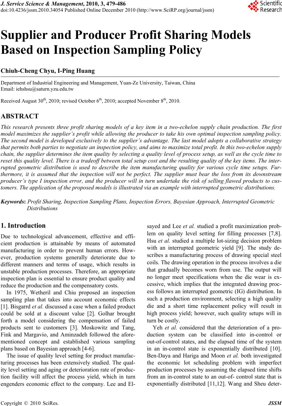J. Service Science & Management, 2010, 3, 479-486
doi:10.4236/jssm.2010.34054 Published Online December 2010 (http://www.SciRP.org/journal/jssm)
479
Supplier and Producer Profit Sharing Models
Based on Inspection Sampling Policy
Chiuh-Cheng Chyu, I-Ping Huang
Department of Industrial Engineering and Management, Yuan-Ze University, Taiwan, China
Received August 30th, 2010; revised October 6th, 2010; accepted November 8 th, 2010.
ABSTRACT
This research presents three profit sharing models of a key item in a two-echelon supply chain production. The first
model maximizes the supplier’s profit while allowing the producer to take his own optimal inspection sampling policy.
The second model is developed exclusively to the supplier’s advantage. The last model adopts a collaborative strategy
that permits both parties to negotiate an inspection policy, and aims to maximize total profit. In this two-echelon supply
chain, the supplier determines the item quality by selecting a quality level of process setup, as well as the cycle time to
reset this quality level. There is a tradeoff between total setup cost and the resulting quality of the key items. The inter-
rupted geometric distribution is used to describe the item manufacturing quality for various cycle time setups. Fur-
thermore, it is assumed that the inspection will not be perfect. The supplier must bear the loss from its downstream
producer’s type I inspection error, and the producer will in turn undertake the risk of selling flawed products to cus-
tomers. The application of the proposed models is illustrated via an example with interrupted geometric distributions.
Keywords: Profit Sharing, Inspection Sampling Plans, Inspection Errors, Bayesian Approach, Interrupted Geometric
Distributions
1. Introduction
Due to technological advancement, effective and effi-
cient production is attainable by means of automated
manufacturing in order to prevent human errors. How-
ever, production systems generally deteriorate due to
different manners and terms of usage, which results in
unstable production processes. Therefore, an appropriate
inspection plan is essential to ensure product quality and
reduce the production and the compensatory costs.
In 1975, Wetheril and Chiu proposed an inspection
sampling plan that takes into account economic effects
[1]. Bisgarrd et al. discussed a case when a failed product
could be sold at a discount value [2]. Golhar brought
forth a model considering the compensation of failed
products sent to customers [3]. Moskowitz and Tang,
Fink and Margavio, and Aminzadeh followed the afore-
mentioned concept and established various sampling
plans based on Bayesian approach [4-6].
The issue of quality level setting for product manufac-
turing processes has been extensively studied. The qual-
ity level setting and aging or deterioration rate of pro duc-
tion facility will affect the process yield, which in turn
engenders economic effect to the company. Lee and El-
sayed and Lee et al. studied a profit maximization prob-
lem on quality level setting for filling processes [7,8].
Hsu et al. studied a multiple lot-sizing decision problem
with an interrupted geometric yield [9]. The study de-
scribes a manufacturing process of drawing special steel
coils. The drawing op eration in the process involves a die
that gradually becomes worn from use. The output will
no longer meet specifications when the die wear is ex-
cessive, which implies that the integrated drawing proc-
ess follows an interrupted geometric (IG) distribution. In
such a production environment, selecting a high quality
die and a short time replacement policy will result in
high process yield; however, such quality setups will in
turn be costly.
Yeh et al. considered that the deterioration of a pro-
duction system can be classified into in-control or
out-of-control states, and the elapsed time of the system
in an in-control state is exponentially distributed [10].
Ben-Daya and Hariga and Moon et al. both investigated
the economic lot scheduling problem with imperfect
production processes by assuming the elapsed time shifts
from an in-control state to an out-of- control state that is
exponentially distributed [11,12]. Wang and Sheu deter-

Supplier and Producer Profit Sharing Models Based on Inspection Sampling Policy 480
mined the optimal lot size with an assumption that the
deteriorating production system has a geometric survival
distribution under a free-repair warranty policy [13].
Wang obtained the optimal lot size by assuming the dete-
riorating productio n process has an increasing failur e rate
with a general shift distribution [14]. Other studies as-
sumed that the number of conforming items in the im-
perfect production process has the following distributions:
discrete uniform [15], binomial [16], and interrupted
geometric [17-19].
This research presents three profit sharing models of a
product involving a key item in a two-echelon supply
chain process. The upstream supplier determines the
quality level and cycle time setting of the key item pro-
duction, while the downstream producer can select its
own inspection sampling plan. It is assu med that the item
manufacturing quality meets the interrupted geometric
distribution, and inspection errors may occur. Bayesian
approach is used to solve the two-echelon benefit prob-
lem by incorporating into the models the following fac-
tors: the supplier’s item quality information, the pro-
ducer’s sampling information, inspection and product
failure costs, and inspection accuracy. Finally, an exam-
ple is provided to illustrate the features and applications
of the models.
The remainder of the paper is organized as follows:
Section 2 defines the problem and describes the model;
Section 3 presents numerical results of two examples;
Section 4 concludes this study.
2. Problem and Models
In this section, notations used throughout the paper are
first introduced. The problem then is illustrated in
Sub-Section 2.2 via a diagram. Finally, three profit shar-
ing models and a sampling inspection plan are detailed in
subsequent sections.
2.1. Notations
x: a process quality level setting, x  X.
X: set of possible quality level settings.
T: cycle time for resetting the process quality lev e l.
 : set of all choices for cycle time T.
Su: selling price per item by supplier.
Cu: manufacturing cost per item by supplier.
Cx: setup cost for process quality level x.
N: quantity ordered by producer.
Sd: selling price per item by producer.
D1: producer’s stage 1 decision for sample size n.
q1: probability of no type I error, a constant.
q2: probability of no type II error, a constant.
P: process yield or probability that an item is good; a
random variable.
W: probability of an item being reported “good” dur-
ing inspection.
Yn: number of reported “defective” items at stage 1; y
is the realization.
ZN-n: number of defective items in the remainder of lot.
YN-n: total number of reported “defective” items in the
remainder of the lot after full inspectio n.
k1: inspection cost per item.
k2: penalty cost of a failed product sold to customers.
M(y): number of inspections to compensate y reported
as “defective” to producer.
R(n): number of defectives due to type II error for n
reported “good” items.
D2: producer’s stage 2 decision on the re mainder of th e
lot after observing the sampling outcome; it con tains two
alternatives: stop inspection (Sn) and continue to inspect
the remaining all (CN).
M(YN-n): number of inspections to obtain YN-n reported
“good” items.
Mcp(x,T,n): number of items to compensate producer
under supplier’s setup (x,T) and producer’s sampling size
n.
2.2. Problem Description
Consider a decision problem arising in a two-echelon
production process, where the upstream level (or supplier)
manufactures a key item and the downstream level (or
producer) assembles a product involving this key item.
The supplier can select the item production process with
a high quality level setup and short cycle time for reset-
ting, but the corresponding total setup cost will be large.
On the other hand, if the supplier selects a low quality
level with large cycle time, the total setup cost is lo w, but
the risk of returned defective items will be high. Fur-
thermore, for both cases the item quality can be im-
proved if the supplier selects a smaller cycle time of re-
setting the produc tion process. The problem assu mes that
the producer bears all inspection cost under its sampling
plan, and the supplier undertakes the compensation cost
of the returned items.
Figure 1 portrays the problem. When the supplier re-
ceives a demand request, he schedules the production
process and determines the initial qu ality setup level “x”,
as well as the cycle time “T” to reset the process. A
higher initial quality level setup will incur a higher cost,
and such will be the same for a shorter cycle time. On the
other hand, the downstream producer can take a
two-stage rectifying inspection before sending items to
its assembly line. Stage 1 determines the sample size,
whereas stage 2 chooses between continuing and stop-
ping the remaining items in the lot after the sampling
utcome is observed. It is assumed that the inspection o

Supplier and Producer Profit Sharing Models Based on Inspection Sampling Policy 481
Figure 1. Diagram of the two parties’ decision problem.
decision on the sample size n for the purchase lot of size
N. Likewise, f2 (x,T,N,n) is the profit received by the
producer under sample size n. Both functions can be ex-
pressed as follows.
will be imperfect; that is, both type I and type II errors
may occur. The supplier bears the risk of type I error,
whereas the producer may suffer a product failure cost
from type II error caused by imperfect inspections. Such
types I and II probabilities are treated as constants and
can be estimated by data and/or according to production
management’s discretion. In summary, the supplier’s
cost includes 1) the quality level setup, 2) the number of
such setups, and 3) reimbursement for items reported
“defective” by the producer. The producer’s cost com-
prises 1) inspection cost for specified sample size n and
extra inspections M(Yn) for compensation of reported
“defective” items, 2) product failure cost due to unin-
spected defective items and/or inspected items with type
II error.





1,, ,
,,
uu
x
cp u
fxTNnS CN
N
CEMxTn
T

 
C


 

(1)
where
x



 is the smallest integer greater than or equal
to x and represents the number of production setups for
this order, and










2
,,
|,Pr |
N
cp n
Nn
yDC
EM xTnEMY
EMY nyyn


 



is the expected number of additional inspections when
the producer’s sampling size is n. This term includes the
extra inspections required to compensate for the reported
“defective” items during stage 1 inspection, and the
number of r eported “d efective” items at stage 2 wh en the
stage 2 decision is to continue inspecting the remaining
items of the lot (Equ a tion 2).
Clearly, the profit-maximizing objectives of the sup-
plier and the producer will conflict. We consider three
models in the next section to resolve this conflict.
2.3. Mathematical Models
It is assumed that the qualities of items in the lot and
items for compensation are statistically independent, and
have a common prior distribution. Furthermore, the sam-
pling information can be applied to calculate the posteri-
ors for both type s of items. where




2sN
LRnZk
n

 is the loss due to decision
“Sn”,


1
N
C
LNnk



1Nn
M
Yk




2
RN k

Let f1(x,T,N,n) denote the profit received by the sup-
plier under its setup decision (x,T), and the producer’s
is
the lo
to decision “CN”, and n + E(M(y)|n,y) is the
expected total number of in spections to obtain n reported
ss due
  



211
0
,, ,|,,|,Pr|
nn
n
duS C
y
f
xTNnSCNnkMyk MinELnyELnyyn


 

 (2)

Supplier and Producer Profit Sharing Models Based on Inspection Sampling Policy 482
“good” items given the sampling result (n,y). The pro-
ducer’s optimal sample size n* is the number satisfying
quation (3). Clearly, f2(x,T,N,n*) is the expected
tio tempts to
m
E
maximum profit that the producer can obtain under
quality level setup (x,T).
Model 1: Producer’s profit maximiz ation
In this model, the producer’s profit maximization is a
constraint (Equation 4) of the supplier’s profit optimiza-
n problem. In other words, the supplier at
aximize its profit by selecting a quality setup (x,T)
given that the producer has optimized its own expected
profit under (x,T).

*
11
,,,
M
aximizefx TNn
, xXT


*
212
,,,,,, for 0
f
xTNnfxTNnnN (4)
Model 2: Supplier’s profit maximization
The supplier’s profit is maximized when the
ducer’s sampling size n is 0; in such a case there w
no
Model 3: Collaborative strategy for total profit
maximization
pro-
ill be
compensation to the producer.

1
,,,0aximizefxTNn 
, xXT
(5)
M



, ,
12
,,,,
M
aximizefx TNnfxTN n
, , 0
x
XTn N (6)
This model permits both parties to negotiate the in-
spection sampling policy to be execuy the pro-
ducer. This collaborative strategy will
m
ted b
yield the maxi-
um total profit as the profit conflict between both sides
is minimized.
For any quality setup (x,T) and requested quantity N,
the following results hold:
1) For Models 1 and 3:
(1.a)

**
12
,,,,,,
f
xTNnfxTNn 

**
112
,,,,,,
1
f
xTNnfxTNn, where n* is the optimal
sample size for Model 3. The reason is th
izes the combined profit f1
, whereas *
1
n optimizes f2 w
at the sample
ithin 0  n siz
 N
e n* optim + f2 w
ithin 0  n  N.
(1.b)

*
2
,,,
f
xTNn 


*
21
,,,
f
xTNn,

*
1
,,,
f
xTNn 

*
11
,,,
f
xTNn and

*
1
,,,
f
xTNn

11
,* , ,
f
xT

,N n  

**
2
,
21
,, ,,
f
xTT N
ls 2 a
N nfxn.




**
12
,, ,,, ,
f
xTNnfxTNn
2) For Modend 3:
(2.a) 




12
,, ,0,, ,0TNnfxTNnfx


(2.b)


*
1,, ,
f
xTNn 

1,, ,0fxTN ,


*
,, ,
2
f
xTNn 


,, ,0TN ad
2
fx n

*
2
,,,
f
xTNn


, ,0N 
1,fxT


22
, ,0,

*
,, ,
f
xTNNf xTn.
2.4. Computation Formulae
The probability that an item is reported as “good” (in-
cluding type II error) is as follows:




1

 




1
1
0
11 pqp
dppwWE
  

02dppq


(7)
where


p 
conform
is the prior probability density function of
an iteming to quality specification. In our study,


p 
is assum
as “d f y ed to be Beta (
 ,  ). The probability o
reported efective” items for n samples is:
 
1
0
Pr |1y
ny
n
ynwwp dp
y




 



Other calculations are shown below.
  
1
0
1
|, |,EM ynyypnydp
w



, whe by

re
Bayes’ theorem we obtain
 
1
|, Pr{ |
y
pn yyn 

}
y
ny
nwwp





 

 
  

12
012
11
|, |,
11
pq
ERnnynpny dp
pqpq












|,1 |,
Nn
E ZnyNnE P ny




 


|,1 |,
Nn
EYnyNnEW ny

 
1
0
|, |,EWnywp nydp 



  
1
|, |,
Nn
EMYnyNn Eny
w





At stage 2, decision “S” is better than “CN” when
n




|, |,
nn
SC
E LnyE Lny. After algebraic opera-
tions, the inequality is converted to

 



|, ,|,Pr
nn
SC

11
0|, |
n
y
0nN
M
innkEMyn ykMinn

 
 ELn yELn yy



(3)


Supplier and Producer Profit Sharing Models Based on Inspection Sampling Policy483

 
2
12
1
2
11
1(|,) |,
11
1|,
Pq
EP nyEny
PqP qk
k
Eny
W
 









(
If there exists an integer c  0 such that for all y > c
decision CN is better than Sn, the integer c will be referred
to as the critical number of sample size n.
2.
y item engen-
erty:ctive item is produced, all items follow-
T
8)
5. Process Quality Level Setup and Cycle Time
Resetting
In the problem, it is assumed that the ke
dered in the production process has the following prop-
once a defe
ing the first defective one will also be defective. Inter-
rupted geometric (IG) distribution meets the item quality
for such a production environment. A short time re-
placement policy of production equipment (resetting)
will result in a high process yield; however, the item
quality enhancement will be costly when the lot size is
large.
For IG, let rx represent the yield of the first item with
respect to x quality level setup. Thus, the probability o f t
non-defective items under cycle time T will be Pr{G = t}
= t(1 )
x
x
rr , t = 0, 2,…, T-1; Pr{ GT = T} = Pr{ GT  T}
= T
x
r. Here we assume that each item takes one unit of
time to produce.
The ae and variance of yield for cycle time T are
as lows:
verag
fol

1
//
1
T
EG T T
r



(9)
T
rr





2
21
2
//
1/
1
1
TT
TT
T
Var GTVar GT
rTr
rT
r
r


2
rT


 
 






For a lot size , the process will perfo
setups to pro. Let be the
number of conf unde
tim yield

(10)
NMT
duce N items
orming items
rm M

1,,M
TT
GG
r M setups with cycle
e T. The expected will be the same as (9), but
the variance becomes



121 2
(...)/ ()/
M
TT TT
VarGGGTMVar GTM

 

(11)
Suppose that the supplier only provides the produce
with information on the mean and variance of the key
item’s quality; if the producer selects Beta (  ,  ) a
pri
an
r
s the
or distribution for the output yield, the parameters 
d  can be estimated by


1/
T
EP EGT




 and (12)

 
 
12 2
/1
T
VarPVar GTM





(13)
3. Illustrative Example
The profit sharing models are illustrat
ple with the following parameters: k1 = 12, k2 = 150, Cu =
120, N = 1500, Su = 180, Sd = 230, two possibilities of
process quality setups: X = {rx | 0.995, 0998}, the set of
resetting cycle times:  = {T | 10, 15, 20, 25, 30},
ty levels: one of whic
and the other two are with
etheless receive
m
creases as true yield E(P), q1, and q2 decrease. The
ed through an exam-
and
h is three cases of inspection quali
error-free (q1,q2) = (1.0, 1.0),
minor errors: (q1, q2) = (0.98, 0.98) and (0.96, 0.96). As
aforementioned, the producer will obtain the mean and
variance of the yield regarding the lot of size N. The pro-
ducer adopts a Beta prior distribution to represent the lot
quality and for sampling inspection. Table 1 presents the
information on yield, E(P) and Var(P), which are derived
from Equations (9), (10) and (11). This information will in
turn be used to estimate the p arameters (
 ,  ) of Beta prior
according to Equations (12) and (13). The results indicate
that a shorter cycle time T leads to a higher item quality
and smaller var iance. The resulting Bet a prior will then be
incorporated with (q1,q2) to calculate “reported good”
probability E(W) using equation (7). Table 2 displays the
probabilities of “reported good” for all possible combina-
tions of {rx, T, (q1,q2)}. The higher the value of (q1,q2), the
larger the probability of “report ed good”.
Table 3 show s the numerical results of the three mod -
els when T = 15 and N = 1500 with three different (q1, q2)
values. The calculation uses the following quality setup
costs: Cx = 450 for rx = 0.995, and Cx = 500 for rx = 0998.
Generally, when there are inspection errors, reported
defective probability 1-E(W) increases as the value of
(q1,q2) decreases. The producer will non
aximum profit in Model 1 as its risk of delivering de-
fective products to customers is minimized. However, the
supplier will receive minimum benefit if he complies
with Model 1. In contrast, the supplier’s profit will be
maximized in Model 2, since he has no obligation for any
defective items sent to the producer. Here, the producer’s
interest is reduced to the minimum. In Model 3, the
benefits of both parties are between Models 1 and 2, but
their combined profit is the highest. In the case of T = 15
and N = 1500, the optimal decisions (rx,n*,c*) are
(0.995,18,0), (0.998,12,0), (0.998,10, 1) for (q1,q2) =
(0.96,0.96), (0.98,0.98) and (1.0,1.0), respectively. It
appears that for any model, the profit of either party de-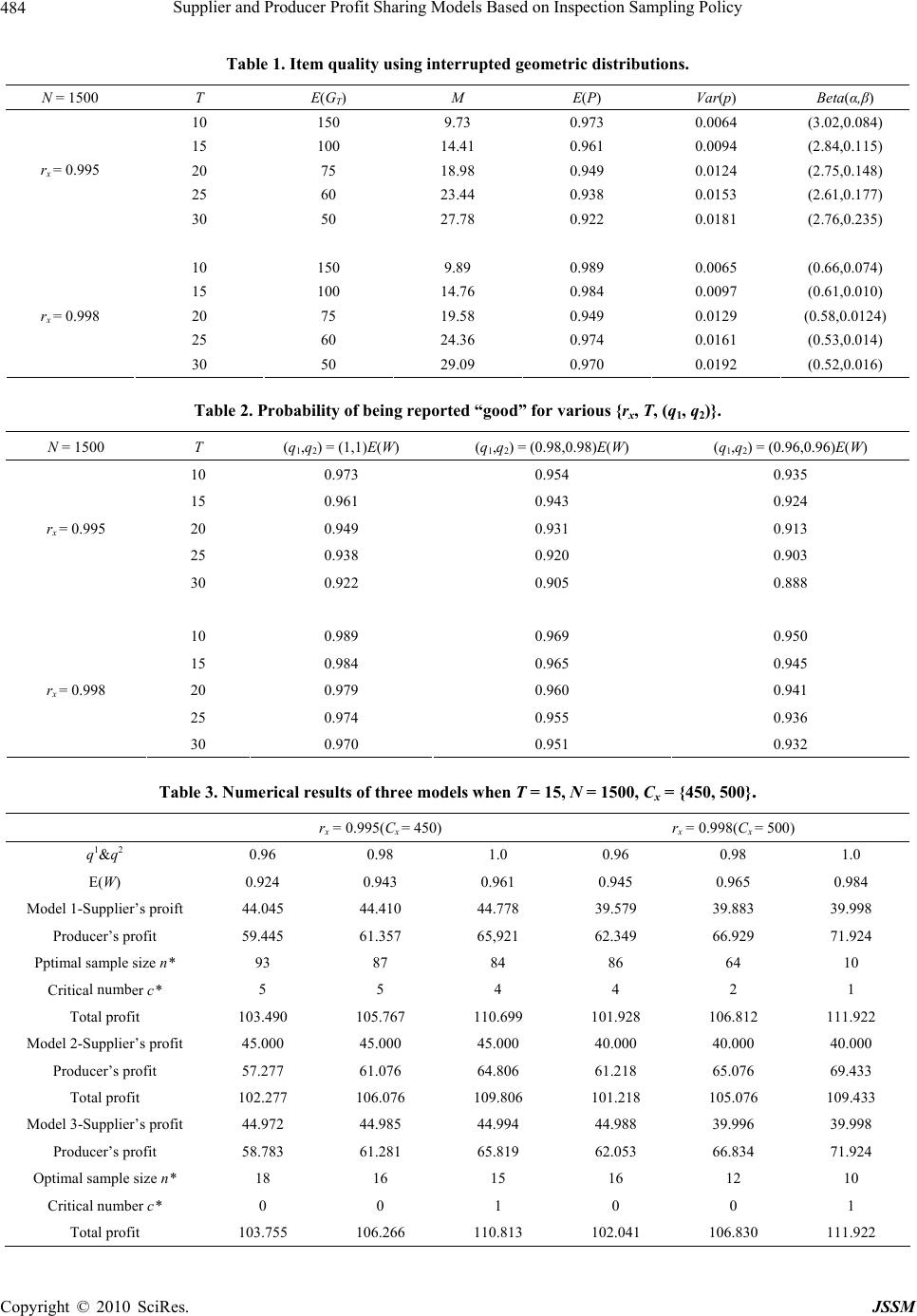

Supplier and Producer Profit Sharing Models Based on Inspection Sampling Policy 484
Table 1. Item quality using intepte d ge ometr i c distr i butions.
N = 1500 T E(GT) M E(P) Var(p) Beta(α,β)
rru
10 150 90.973 0.0064 (3.02,0.084) .73
15 100 14
20
rx = 0.995
.41 0.961 0.0094 (2.84,0.115)
0124 (2.75,0.148)
25 60 23.44 0.938 0.0153 (2.61,0.177)
2 (
rx = 0.998
30 50 29. 0.970 0.0192 (0.52,0.016)
75 18.98 0.949 0.
30 50 7.780.922 0.0181 2.76,0.235)
10 150 9.89 0.989 0.0065 (0.66,0.074)
15 100 14.76 0.984 0.0097 (0.61,0.010)
20 75 19.58 0.949 0.0129 (0.58,0.0124)
25 60 24.36 0.974 0.0161 (0.53,0.014)
09
ble 2. Probabf being reported “good” for v {rx, T, (q1,
N = 1500 (q1,q21,1)E(W) 1,q2) = (0.98,W) ) = (0.96,
Taility oarious q2)}.
T ) = ((q0.98)E((q1,q20.96)E(W)
10 0.973 0.954 0.935
15 0.961 0.943 0.924
0.913
rx = 0.995
25 0.974 0.955 0.936
rx = 0.998
20 0.949 0.931
25 0.938 0.920 0.903
30 0.922 0.905 0.888
10 0.989 0.969 0.950
15 0.984 0.965 0.945
20 0.979 0.960 0.941
30 0.970 0.951 0.932
Tab Numerical res three models when T = 15, = 1500, Cx = {450, 500}.
5(Cx = 450) r
x = 0.998(Cx =
le 3.ults ofN
rx = 0.99 500)
q1&q2 0.96 0.98 1.0 0.96 0.98 1.0
E(W) 0.924 0.943 0.961 0.945 0.965 0.984
Model 1-Supplier’s pr39.998
Produces profit 59.445 65,921 62.349 71.924
Pptimal size n*
Criticaer c*
Mo
5 6 6 6 6 6
1077 106 106 108 106 103
Modelofit
Op
Cri c*
oift 44.045 44.410 44.778 39.579 39.883
r’61.357 66.929
sample 93 87 84 86 64 10
l numb5 5 4 4 2 1
Total profit 103.490 105.767 110.699 101.928 106.812 111.922
del 2-Supplier’s profit 45.000 45.000 45.000 40.000 40.000 40.000
Producer’s profit 7.2771.0764.8061.2185.0769.433
Total profit 2.26.079.801.215.079.43
3-Supplier’s pr44.972 44.985 44.994 44.988 39.996 39.998
Producer’s profit 58.783 61.281 65.819 62.053 66.834 71.924
timal sample size n* 18 16 15 16 12 10
tical number 0 0 1 0 0 1
Total profit 103.755 106.266 110.813 102.041 106.830 111.922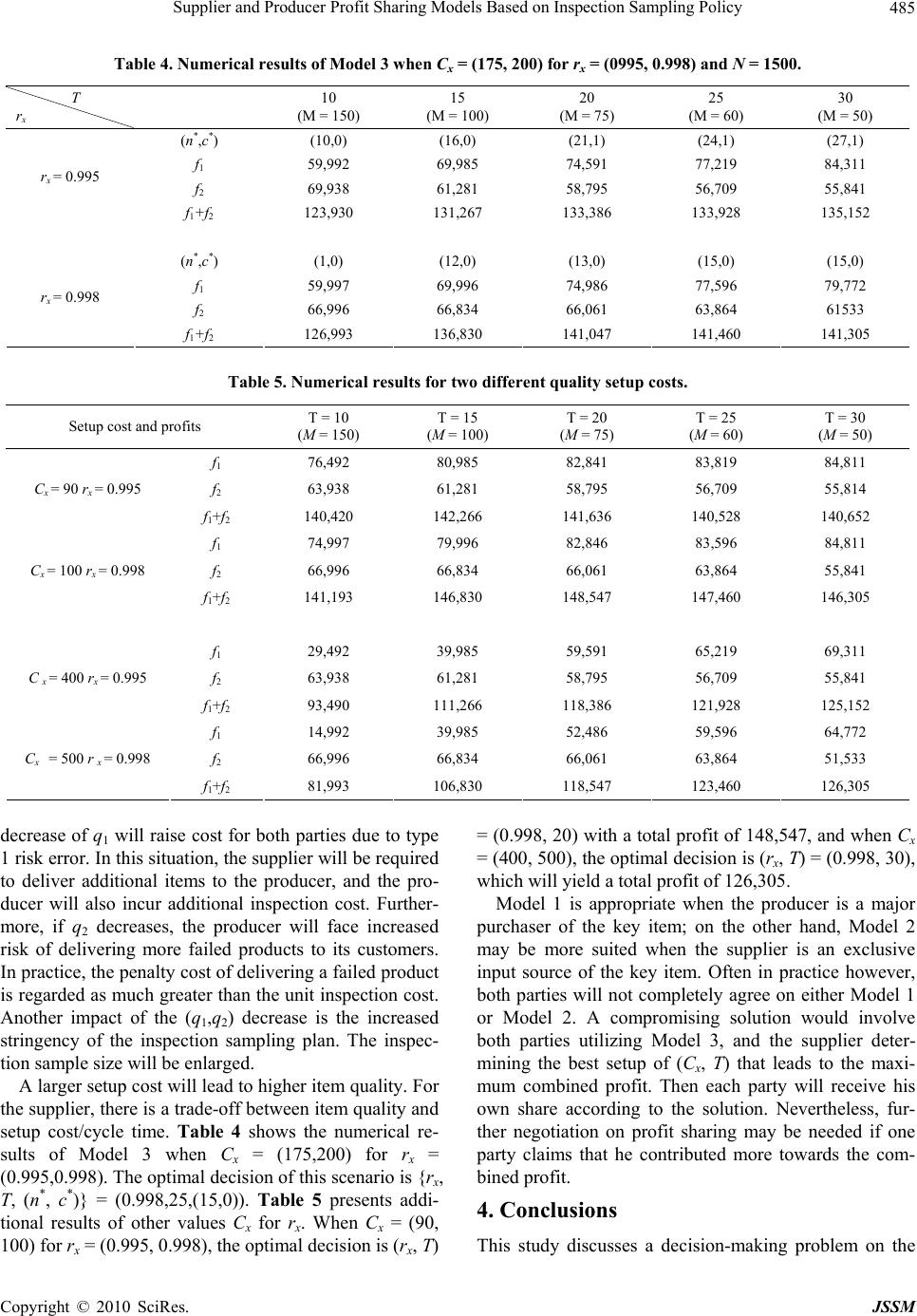

Supplier and Producer Profit Sharing Models Based on Inspection Sampling Policy485
. Numericlts of Moen Cx = (175, 200) for rx , 0.998) a1500.
rx 10 (M = 150) 15 (M = 100)20 (M = 7525 (M = (M = 50)
Table 4al resudel 3 wh= (0995nd N =
T ) 60) 30
(n*,c*) (10,0) (16,0(21,() 1) 24,1) (27,1)
f1 59,992 69,985 74,591 77,219
f 69,938 61,281 58,795 56,709 55,
84,311
2841
rx = 0.995
f1 2
x
+f 123,930 131,267 133,386 133,928 135,152
(n* *) ,c(1,0) (12,0) (13,0) (15,0) (15,0)
f1
f
59,997 69,996 74,986 77,596 79,772
2 66,
f1+f2
996
126,993
66,834
136,830
66,061
141,047
63,864
141,460
61533
141,305
r= 0.998
Table 5. Nu results foifferent quetup costs.
Setup cost and profi
mericalr two dality s
ts T = 10
(M = 150) T = 15 (M = 100) T = 20 (M = 75) T = 25 (M = 60) T = 30 (M = 50)
f1 76,492 80,985 82,841 83,819 84,811
f26,709 55,814
Cx = 90 rx = 0.995
f1+f2 140,142,141,
f1
Cx = 100 rx = 0.998
f
f1 14,992 39,5 52,486 59,596 64,772
Cx = 500 r x = 0.998
f
63,938 61,281 58,795 5
420
74,997
266
79,996
636 140,
82,846
528 140,
83,596
652
84,811
f2 66,996 66,834 66,061 63,864 55,841
1+f2141,193 146,830 148,547 147,460 146,305
f1 29,492 39,985 59,591 65,219 69,311
f2 63,938 61,281 58,795 56,709 55,841 C x = 400 rx = 0.995
f1+f2 93,490 111,266 118,386 121,928 125,152
98
f2 66,996 66,834 66,061 63,864 51,533
1+f281,993 106,830 118,547 123,460 126,305
decrease of q1 will raise coboth pue to typ
1 risk ation the supplier e required
to dms to the produd the pro-
ducer will also incur additional inspectrther
ore, if q decreases, the producer will face increased
n of this scenario is {r,
T,
(0.998, 2 a total pr148,547, en Cx
400, 500)ptimal decisio( rx, T) = , 30),
ich will yielotal profit ,305.
Model 1opriate w produceajor
purchaser of the key item; on the other hand, Model 2
rtheless, fur-
th
st for arties de =
error. In this situ
eliver additional ite,will b cer, an
ion cost. Fu-
m2
risk of delivering more failed products to its customers.
In practice, the penalty cost of deliv ering a failed product
is regarded as much greater than the unit inspection co st.
Another impact of the (q1,q2) decrease is the increased
stringency of the inspection sampling plan. The inspec-
tion sample size will be enlarged.
A larger setup cost will lead to higher item quality. For
the supplier, there is a trade-off between item quality and
setup cost/cycle time. Table 4 shows the numerical re-
sults of Model 3 when Cx = (175,200) for rx =
(0.995,0.998). The optimal decisiox
(n*, c*)} = (0.998,25,(15,0)). Table 5 presents addi-
tional results of other values Cx for rx. When Cx = (90,
100) for rx = (0.995, 0.998), the optimal decision is (rx, T)
may be more suited when the supplier is an exclusive
input source of the key item. Often in practice however,
both parties will not completely agree on either Model 1
or Model 2. A compromising solution would involve
both parties utilizing Model 3, and the supplier deter-
mining the best setup of (Cx, T) that leads to the maxi-
mum combined profit. Then each party will receive his
own share according to the solution. Neve
0) withofit of and wh
= (
wh , the o d a tn is of 126(0.998
is apprhen ther is a m
er negotiation on profit sharing may be needed if one
party claims that he contributed more towards the com-
bined profit.
4. Conclusions
This study discusses a decision-making problem on the

Supplier and Producer Profit Sharing Models Based on Inspection Sampling Policy 486
profit sharing of a key item in a two-echelon supply
chain process. The upstream supplier determines the
quality level, as well as the reset cycle time, during the
manufacturing process. However, the producer aims to
minimize his risk by selecting and implementing an op-
timal inspection decision. Since the two parties have
conflicting interests, three profit sharing models are pro-
e conflict. Model 1 allows the
sk to the minimum level, wh
r and L. Pallesen, “Economic
anufactured Product,”
ntents
for a Canning Problem,” Journal of Quality Technology
Vol. 19, No. 2
tion in Statistics – The-
Engineering, Vol. 57, No. 3, 2009, pp. 699-
120, No.
pp. 875-881.
. 6, 2002, pp. 620-629.
and S. M. Guu, “The Multiple Lot Sizing
ang, “The Finite Multiple Lot
posed to resolve th
ducer to reduce his ripro- ereas [9] H. M. Hsu, T. S. Su, M. -C. Wu and L. -C. Huang, “Mul-
tiple Lot-Sizing Decisions with an Interrupted Geometric
Yield and Variable Production Time,” Computers and
Industrial
Model 2 will work solely to the supplier’s favor. Model 1
will be useful if the producer’s penalty cost of product
failure is high. On the other hand, Model 2 is more ap-
plicable if the supplier provides high quality key items,
or is the dominant source of the key item. These two
models tend to be more one-sided, situation-based solu-
tions that lopsidedly favor either the supplier or producer.
Model 3 may be the most practical and compromising
one, as it requires both parties to work together in ob-
taining the largest sum of profits, and prevents an unrea-
sonably large gap between their individual profits. This
collaborative manufactur ing strategy can ensure that both
parties receive acceptable returns and maintain long-term
business cooperation.
5. Acknowledgements
This work was supported by the National Science Coun-
cil in Taiwan under grant NSC 96-2628-E155-006.
REFERENCES
[1] G. B. Wetherill and W. K. Chiu, “A Review of Accep-
tance Sampling Schemes with Emphasis on the Economic
Aspect,” International Statistical Review, Vol. 43, No. 2,
1975, pp. 91-210.
[2] S. Bisgaard, W. G. Hunte
Selection of Quality of MTech-
,
[16] D. W. Pentico, “An Evaluation and Proposed Modifica-
tion of the Sepehri-Silver-New Heuristic for Multiple Lot
Sizing under Variable Yield,” IIE Transactions, Vol. 20,
No. 4, 1988, pp. 360-363.
nometrics, Vol. 26, No. 1, 1984, pp. 9-18.
[3] D. Y. Golhar, “Determination of the Best Mean Co
, 1987, pp. 82-84.
[4] H. Moskowitz and K. Tang, “Bayesian Variables Accep-
tance-Sampling Plans: Quadratic Loss Function and Step-
Loss Function,” Technometrics, Vol. 34, No. 3, 1992, pp.
340-347.
[5] R. L. Fink and T. M. Margavio, “Economic Models for
Single Sample Acceptance Sampling Plans, No Inspec-
tion, and 100 Percent Inspection,” Decision Sciences, Vol.
25, No. 4, 1994, pp. 625-653.
Prob
[6] M. S. Aminzadeh, “Bayesian Economic Variable Accep-
tance-Sampling Plan Using Inverse Gaussian Model and
Step-Loss Function,” Communica
ory and Methods, Vol. 32, No. 5, 2003, pp. 961-982.
[7] M. K. Lee, S. H. Hong and E. A. Elsayed, “The Optimum
Target Value under Single and Two-Stage Screenings,”
Journal of Quality Technology, Vol. 33, No. 4, 2001, pp.
506-514.
[8] M. K. Lee and E. A. Elsayed, “Process Mean and
Screening Limits for Filling Processes under Two-Stage
Scr- eening Procedure,” European Journal of Operation
Research, Vol. 138, No. 1, 2002, pp.118-126.
706.
[10] R. H. Yeh, W. T. Ho and S.T. Tseng, “Optimal Produc-
tion Run Length for Products Sold with Warranty,”
European Journal of Operational Research, Vol.
3, 2000, pp. 575-582.
[11] M. Ben-Daya and M. Hariga, “Economic Lot Scheduling
Problem with Imperfect Production Processes,” The Jour-
nal of the Operational Research Society, Vol. 51, No. 7,
2000,
[12] I. Moon, B. C. Giri and K. Choi, “Economic Lot Sched-
uling Problem with Imperfect Production Processes and
Setup Times,” The Journal of the Operational Research
Society, Vol. 53, No
[13] C. H. Wang and S. H. Sheu, “Optimal Lot Sizing for
Products Sold under Free-Repair Warranty,” European
Journal of Operational Research, Vol. 149, No. 1, 2003,
pp. 131-141.
[14] C. H. Wang, “The Impact of a Free-Repair Warranty
Policy on EMQ Model for Imperfect Production Sys-
tems,” Computers & Operations Research, Vol. 31, No.
12, 2004, pp. 2021-2035.
[15] S. Anily, “Single-Machine Lot-Sizing with Uniform
Yields and Rigid Demands: Robustness of the Optimal
Solution,” IIE Transactions, Vol. 27, No. 5, 1995, pp.
625-633.
[17] S. Anily, A. Beja and A. Mendel, “Optimal Lot Sizes
with Geometric Production Yield and Rigid Demand,”
Operations Research, Vol. 50, No. 3, 2002, pp. 424-432.
[18] A. X. Zhang
lem with Rigid Demand and Interrupted Geometric
Yield,” IEE Transactions, Vol. 30, No. 1, 1998, pp. 427-
431.
[19] S. M. Guu and A. X. Zh
Sizing Problem with Interrupted Geometric Yield and
Holding Costs,” European Journal of Operational Res-
earch, Vol. 145, No. 3, 2003, pp. 635-644.