Applied Mathematics
Vol.3 No.10A(2012), Article ID:24120,11 pages DOI:10.4236/am.2012.330210
Portfolio Selection under Condition of Variable Weights
College of Mathematical Sciences, Isfahan University of Technology, Isfahan, Iran
Email: r.keykhaei@math.iut.ac.ir, jahandid@cc.iut.ac.ir
Received July 11, 2012; revised August 9, 2012; accepted August 16, 2012
Keywords: Mean-Variance Optimization; Riskless Asset; Efficient Frontier; Free Asset
ABSTRACT
In this paper we generalize the single-period Markowitz Mean-Variance portfolio selection problem. The Markowitz’s model requires that after choosing the number of each security which constructs the portfolio in the beginning of the investment period, these numbers remain constant during and at the end of the investment period. We drop this assumption and consider an investment model in which the number of each security can vary randomly during the investment period. Indeed we consider a single-period investment with the property that the initial weight of each security is not equal to the final weight of that security. We redefine the notion of the rate of return of each security and show that the return of the investment in a cash account is not certain. We investigate some alternatives among risky securities which acts similar to cash accounts. For this we introduce the notion of free security and relate free securities to a riskless security.
1. Introduction
After that Markowitz [1] originated the Modern Portfolio Theory (MPT) by introducing his single-period MeanVariance (M-V) portfolio selection problem in 1952, many authors have worked on this field. Markowitz considered a portfolio of risky asset. In 1958 Tobin [2] introduced the notion of riskless asset when he entered cash account in his portfolio and stated the one-fund theorem. This theorem says that when both borrowing and lending at the riskless rate are allowed, there is a single risky fund such that every efficient portfolio (portfolios whose expected returns are largest among all portfolios with the same variance) can be constructed as a combination of the fund and the riskless asset. In the Mean-Standard Deviation space, the efficient portfolios can be represented by a straight line which is called the optimal Capital Allocation Line (CAL) (see Tütüncü [3]). In 1972, Merton [4] described the mathematics of the efficient portfolios in full analytic approach. The geometric viewpoint of the MeanVariance analysis was developed by Merton [4] and Roll [5]. There are a huge contributions about asset allocation problem. Recently Steinbach [6] in a survey paper has a complete review on the different models in this case.
In the classic one-period M-V portfolio selection problem, the weight assigned to each security contained in portfolio has been considered to be constant. In other words, if someone at the beginning of the investment period (t = 0) enters in the capital market with initial wealth  and invest his/her wealth as
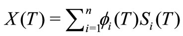
between n securities, then his/her wealth at the end of the investment period ( ) is
) is
 where
where  and
and  are, respectively, the value of the ith security at the beginning and the end of the period, and for each i, fi is the number of shares of the ith security. Here,
  is nondeterministic and is considered to be a random variable, although, at the beginning and at the end of the investment period, fi’s remain fixed.
In our model, we assume that fi’s are nonconstant and vary randomly. In fact it is possible that  for some i, where for each i,
  is the number of shares of the ith security at the beginning of the period and
  is the number of the same one at the end of the period. Thus the value of portfolio at the beginning of the period is
and at the end of the period, it is
 .
.
We can interpret the changes in the values of the fi’s as follows. Consider an investor who has this opportunity to receive some amount of the ith security, as a gift or a reward, during the investment period (after constituting his initial portfolio), it is possible that he/she loses some amount of the ith security by a contract that force him/her to pay his obligation via the ith security. This variability is more plausible in the commodity markets. One who intends to invest his/her wealth on the commodities, some activities such as holding and transporting of commodities impose additional risks; besides other commodity risks, caused by natural or accidental events, on the investment. If we consider the occurrence of the above events as a possibility, then the value of  will be a random variable.
The importance of our model can be seen in the following conditions:
● There is someone who is willing or is forcing to make an investment by imposing some obligations in his/her portfolio investment;
● There might be no possibility or willing to insure the commodities included in the investment;
● Moreover, since this model generalizes the Markowitz model, we can use the obtained results in the classic portfolio selection problems.
It is important to note that although the essence of , as a random variable, is common between all investors, but the nature of
  is special for each investor and can vary from one investor to another. Thus we fit our model to a special investor who wants to construct the optimal portfolio by considering the fact that the security weights can vary randomly.
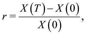
Under this new assumption, we want to develop the notion of one-period Markowitz portfolio selection problem. On the other hand, we know that in the classic MeanVariance analysis (with invariable weights), the rate of return of each security  and the rate of return of the portfolio r are defined. Then the mean and the variance of r are set the criteria for choosing the optimal portfolio. Indeed
  and r are defined as follow:
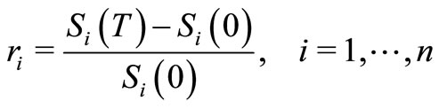 (1)
(1)
and
 (2)
(2)
then
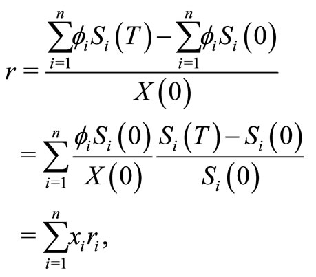
in which
 (3)
(3)
Clearly
 .
.
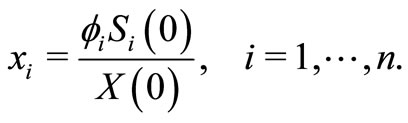
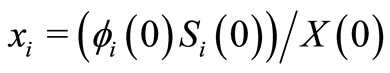
Indeed for each i,  is the the assigned weight allocated to the ith security in the portfolio. Here we denote each security by its weight and the portfolio by the vector of security weights. Thus
  and
and
denote the ith security and the portfolio, respectively. Obviously in the case that fi’s are invariable, ’s are also invariable and for variable fi’s,
 ’s are variable. The M-V portfolio selection problem minimizes the variance of r, subject to a desired mean return ρ. Indeed the problem leads to the following quadratic programming problem which its solution is known:
Problem .
.
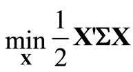
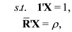
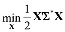
where  is the covariance matrix of the security returns and
  is the vector of mean returns
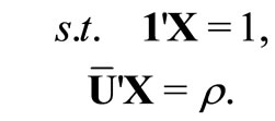
 . Also 1 is the n-column vector of ones.
This paper is organized as follows: In Section 2, we introduce the model and its formulation. The connection between free securities and riskless assets is investigated in Section 3. In Section 4, we describe the relation between a set of free securities with both a free security and a riskless security.
2. Portfolio with Variable Weights
Now we want to know how we should state the portfolio selection problem with variable weights so that we can apply the standard methods to solve it (see Theorem 2.5). To do this, we show that, if an investment asset has any additional benefits beyond capital gains such as random growths or losses of shares, then returns should be adjusted to include any additional components of returns. As the first step, it is necessary to determine the increments of the number of shares for each security.
Definition 2.1. For a portfolio with variable weights, let for each i,
where  and
and  are the number of security
  at the beginning and at the end of the period, respectively. We call
  the rate of increments of
 .
.
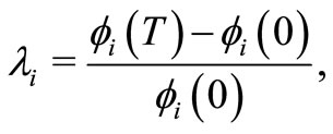
Example 2.2. Assume that an event occurs according to a Poisson process  with rate λ, and for any arrival, the investor obligate to pay one share of the ith security, where i is fixed. Then at the end of the investment period
 , with
 ,
,
Thus  is a nonpositive random variable such that
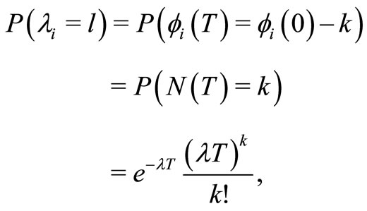
for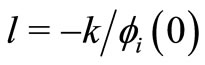 , where
 .
.
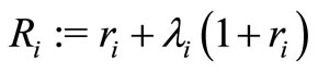
By applying the above definition and (2), we have
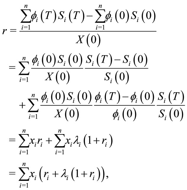
for
as the initial weight allocated to the ith security. r can be written as
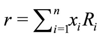 where
where
 .
.
Definition 2.3. Let for each ,
,  be the rate of the return of the security
 . We define
 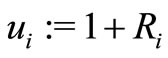 and
and
as the total-return of  and the total-return (or briefly the return) of the portfolio, respectively.
Note. Suppose we possess one share of the ith security. By considering its total-return , at the end of the period, its value becomes
 as expected, since
  is the number of this security. Also,
Now we can state our portfolio selection problem in the form of the problem . Assume that all the securities are risky and
  is the n-column random vector and
  is the covariance matrix of the totalreturns
 . Also, define
  as the n-column vector of mean total-returns
  of these n securities. The mean and covariance matrix of the totalreturns are assumed to be known. By these assumptions, the portfolio selection problem with variable weights can be stated in the following form:
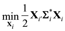
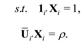
Problem 1. Consider the desired mean total-return ρ for the portfolio. Our aim is to solve the following Mean-Variance portfolio selection problem,
Assumptions. The imposed assumptions on the problem are as follows:
● (A.1) The covariance matrix  is positive definite.
● (A.2) The mean vector  is not a multiple of 1.
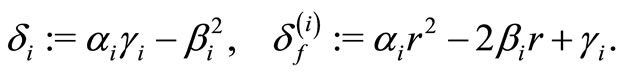
The following constants are frequently used in the sequel and we define them similar to those defined in [6] as follows:
 (4)
(4)
Lemma 2.4. The constants α, γ and δ are positive.
Proof. See Lemma 1.3 of [6].
In the above lemma we realized that we can not specify the exact rang of β. Indeed β may not be positive.
By applying the Lagrangian multiplier method, we can interpret the solution of Problem 1. In the following we display the primal-dual solution of Problem 1 by . Also
  denotes the optimal variance of the problem, which is the variance of the solution. Like [6], we call the whole graph of the optimal variance the efficient frontier.
Theorem 2.5. Problem 1 has the unique primal-dual solution
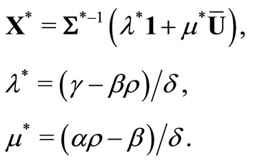 (5)
(5)
Also the optimal variance is
 (6)
(6)
Proof. See Theorem 1.5 and Theorem 1.7 of [6].
Note. Although it seems that the variability of the weights complicates the portfolio selection problem, we see that the problem can be converted to the classical form of portfolio selection problem with invariable weights (Problem ) by using the notion of totalreturns. Therefore, we can employ most of the results for portfolio selection in the situation of invariable weights to the case of variable weights. Clearly when
 1
1
for each , then we have a portfolio selection problem with invariable weights. Thus our model can be interpreted as an extension of classical M-V optimization problem.
3. Existence of Riskless Securities
Note that a security is riskless, if its return is guaranteed and hence it is deterministic. Although cash accounts are commonly considered as riskless securities, in our model they are not riskless. Because of the change in weights, the amount of the gain for a cash account is not deterministic. Indeed the variance of its total-return is not zero. Now we redefine the notion of riskless security on the bases of its total-return.
Definition 3.1. We say a security is riskless, if the variance of its total-return is zero and denote it by its weight .
.
By the above definition, a cash account is riskless if and only if the rate of its increments is constant. In addition, it is not necessary for a riskless security to be of the form of a cash account.
As mentioned above, in our model, it is rare that a portfolio contains a riskless security. In the following, we try to find some risky securities which act like riskless securities to improve our model. Clearly this can also be applied for M-V portfolio selection with invariable weights.
Definition 3.2. Let the total-return of a risky security be uncorrelated with the total-return of all securities in a set of risky securities S. We call such a security free (with respect to S) or S-free; and display it and its total-return by  and
and , respectively.
Example 3.3. We investigate the correlation coefficients between the weekly rate of returns of a set of stocks chosen from S & P500: AEP, ARG, BMY, CPB, DPS, DUK, ERTS, LH, LLY, MCD, MKC, PGN, PPL, SCG, SO, SWY, UNH, WAG, WAT, WDC, WEC, WFV, WLP, WPI, WPO, WYNN, YHOO, YUM, ZION, ZMH. The data consist of daily closing stock prices over 2 years period from 3/12/2009 to 3/11/2011. We choose two assets ARG and WEC, which have low correlation coefficients with the other assets and present the correlation coefficients between their rate of returns and the rate of returns of the other assets in Table 1.
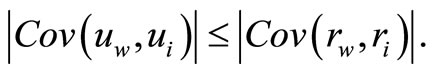
Suppose we can construct a portfolio for which the rate of increments of each asset has a mean in , is independent of the rate of return of that asset and it is independent of the rate of increments and the rate of returns of the other assets. Let us say two random variables are uncorrelated if the absolute value of their estimated correlation coefficient is less than 0.1 (at a significant level grater than 0.05). Now we can observ from Table 1 that for a weekly investment, the stock WEC is S-free, where S = {ARG, BMY, CPB, DPS, LH, MKC, PPL, UNH, WAT, WDC, WFV, WLP, WPI, WYNN, YHOO, YUM, ZION, ZMH}, since, for WEC with the total-return
  and the ith asset of S with the total return
 , we have
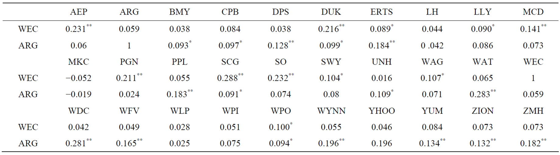
Table 1. Estimated values of correlation coefficients.
where ,
,  ,
,  and
and . So,
. So,
Also, the stock ARG is S-free, where S = {AEP, LH, MCD, MKC, PGN, SWY, SO, WAG, WEC, WLP, WPI}. The correlation coefficients denoted by * and ** are significant at a (2-tailed) level less than or equal to 0.05 and 0.01, respectively. In the other cases the significant levels are grater than 0.05.
3.1. Portfolio with Risky Securities and One Free Security
Let a portfolio consists of  risky securities
  and a free security
 . Indeed the portfolio can be presented as
 , where
 . For convenience, throughout the paper, we sperate the free securities from other risky securities and call X and
  the “risky part” and the “free part” of the portfolio and denote the portion of each part that appears in the primal solution by “risky solution” and “free solution”, respectively. Let
  be the random vector of total-returns and
  be their covariance matrix. Also let
and  be the
  -column vectors of ones. In the sequel
  and
and  refer to the risky part of the portfolio.
Now our situation is a special case of Problem 1 with one additional risky security  and it can be stated as a new problem:
Problem 2.
Assumptions. Here the assumptions are (A.1) and
● (A.3) The mean vector  is not a multiple of
 .
.
Note. We fix these assumption throughout the paper.
Let
and
 .
.
We define the corresponding constants which are stated in (4) by:
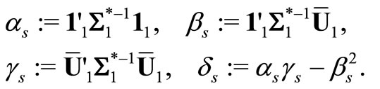
Obviously
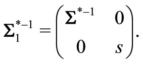
Now
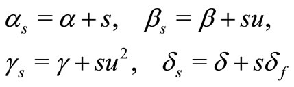 (7)
(7)
where  and
and 2and α, β, γ and δ are related to the risky part of the portfolio and are denoted by (4).
First, consider  as a variable, what will happen when
  decreases to zero or equivalently when s increases to infinity. More precisely, what is the behavior of the solution or the efficient frontier of Problem 2 when the variance of
  tends to zero. Although in our model there is no riskless cash account, by choosing assets with small variances, we show that one can get similar results in contrast with the case that we have riskless cash account. That is, the solution and the optimal variance of the problem converge to the solution and optimal variance in the case where the portfolio contains riskless security. Then with a little connivance, instead of a riskless security, we can use a risky (free) security such that its total-return has the same mean with the cash account and its variance is close to zero. In fact if we consider
  as a variable, then the primal-dual solution and the efficient frontier are functions of the variable
  and to reach our aim, it is sufficient to show that they are continuous functions of
 . First, we investigate the solution of problem 2 when
 .
.
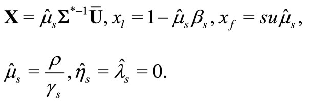
Theorem 3.4. Let . Then, Problem 2 has the primal-dual solution as follows:

Also, the optimal variance is

Proof. See Theorem 1.8 of [6].
Theorem 3.5. The primal-dual solution and optimal variance of Problem 2 are continuous with respect to  3.
3.
Proof. Let . By Theorem 2.5, the corresponding primal-dual solution of the problem for each
is
 (8)
(8)
 (9)
(9)
Then,
 (10)
(10)
Also the optimal variance is
 (11)
(11)
By Lemma 2.4,  is positive. Thus the assertion holds for
 .
.
Let . By Theorem 3.4, Problem 2 has the primal-dual solution
 (12)
(12)
 (13)
(13)
and the optimal variance
 (14)
(14)
To verify the assertion at , substitute the values in (7) in Equations (9)-(11) and take limit when
  goes to zero or equivalently when
  goes to infinity and compar the results with Equations (12)-(14). Now the assertion holds.
Corollary 3.6. Let a portfolio of risky securities contains a cash account  for which its rate of increments
  is uncorrelated with the total-return of the other securities. If the variance of
  converges to zero, then the primal-dual and the optimal variance of the M-V portfolio selection problem converges to the same values for which
  is replaced by a riskless cash account
  with the same mean total-return.
Proof. Assume  is the portfolio. Also, let
 , and
, and  be the rate of return and total-return of
 , respectively. Then
for . Thus
  is a free asset and the assertion holds by Theorem 3.5.
From now on, suppose  and
and  are the primal solution and optimal variance of Problem 2 when
 , respectively (see Equations (13) and (14)).
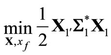
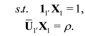
3.2. Portfolio with Risky Securities: A Free Security and a Guaranteed Total Loss
Following section 1.3 of [6], consider a portfolio with  risky securities
  and a security
  with guaranteed total loss, i.e.
 . In this case the portfolio will be
 , where X is the risky part of the portfolio. Since
  is not risky then all covariances associated with
  vanishes. Then the mean and the variance of the total-return of the portfolio become
  and
and , respectively. To eliminate arbitrage opportunity, we impose the additional constraint
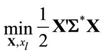
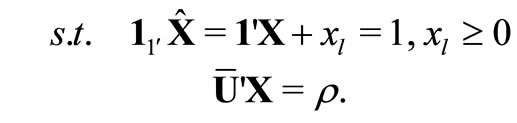
 . With this conditions the problem can be stated as follows:
Problem 3.
We apply the Karush-Kuhn-Tucker conditions to solve the above problem. To do this, let η be the multiplier of the nonnegativity constraint .
.
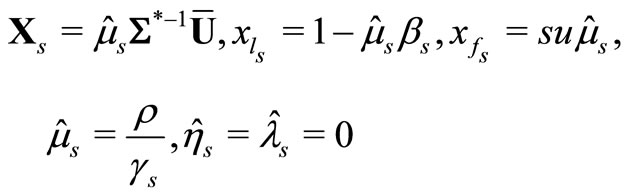
Theorem 3.7. Problem 3 has the following unique primal-dual solution:
1) If , then
a) For ,
,  ,
,  , and
, and  are the same as in the primal-dual solution of Problem 1.
b) For ,
,
2) If , then

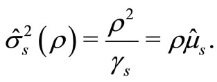
Note that the optimal variance in conditions 1) b) and 2) is
 (15)
(15)
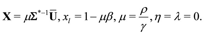
Proof. The Lagrangian associated with Problem 3 is
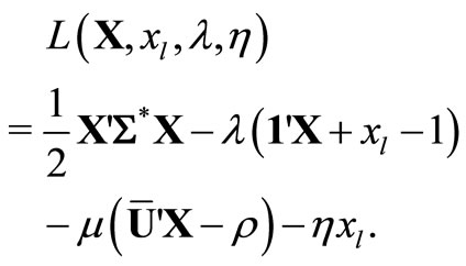
We can consider the system of necessary conditions for the problem as follow:
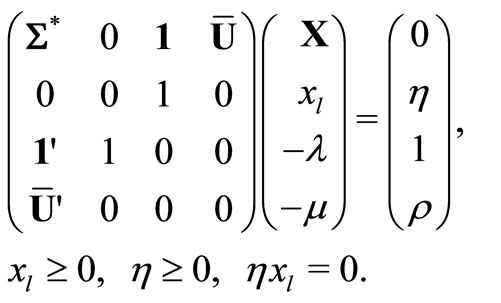
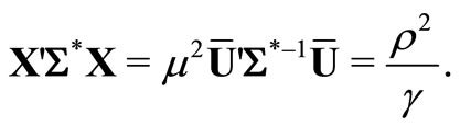
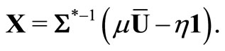
Solving the above system results in 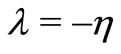 and
and
Consider the condition . If
. If , then we have
  and
and

Thus
So
 (16)
(16)
If , then
  as in Problem 1. Then for
 ,
,
 (17)
(17)
Note that  and δ are positive by Lemma 2.4. Now the proof of the Theorem:
Let , and let
 . If
. If , then
  is negative by (16). On the other hand, if
 , then by (17) the value of λ will be negative, and hence η is positive. Also for
 ,
,  yields that λ is positive and therefore
  is negative, whereas when
 ,
,  is positive. For
 ,
, . So part (1) holds.
Let , since we assume that ρ is nonnegative then the positivity of γ implies that ρ is greater than
 . In this case for
 ,
,  and then η is negative, whereas if
 , then
 .
.
Finally let , then
  leads to positivity of λ and then negativity of η. On the other hand
  yields
  and finally part 2) holds. Uniqueness of the solution follows from strong convexity of the objective function and full rank of the constraint.
In the following; we denote the primal-dual solution of Problem 3 by ; and
; and  as the optimal variance of the problem.
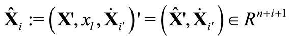
Now consider a portfolio that contains n risky assets ,  and
and . Let
. Let
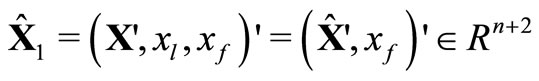
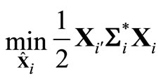
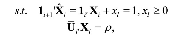
denotes the portfolio. With these assumptions Problem 3 has a new version as follows:
Problem 4.
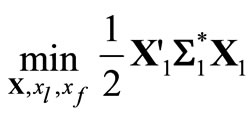
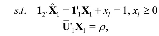
where  is a
is a  -column vector of ones. We display the primal-dual solution of Problem 4 by
 .
.
Corollary 3.8. Problem 4 has the following unique primal-dual solution:
1) If , then
a) For ,
,  and
and  and
and  are identical to the primal-dual solution of Problem 2.
b) For ,
,

2) If , then
Proof. Rearrange the portfolio  to
to , where
 . Now apply Theorem 3.7 for the portfolio
  and use the definition of
 .
.
In order to apply Corollary 3.8, specification of sign of  is necessary. The value of β has the main role in determining the sign of
 . For example when
 , only part 1) of Corollary 3.8 gives the answer, whereas for negative β, both parts of the Corollary can be applied.
In the following let
denote the primal-dual solution of Problem 4 when  which are stated as follows:
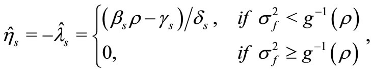
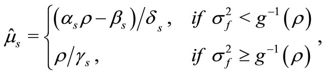
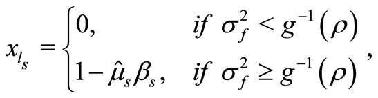
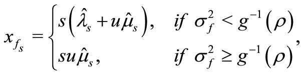
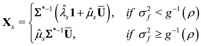
Proposition 3.9. If , then
  and
and  and otherwise
 ,
,
 and
and  is identical to the primal-dual solution of Problem 2, when
 . Also for
 ,
,
 (18)
(18)
Proof. See Theorem 1.12 of [6].
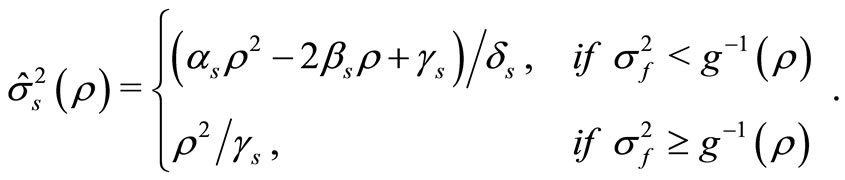
We show the optimal variance of Problem 4 when  by
by  that is
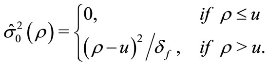 (19)
(19)
Theorem 3.10. The primal-dual solution and optimal variance of the Problem 4 are continuous with respect to .4
.4
Proof. Define the function g by
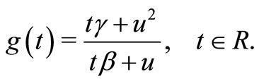
Observe that for any ,
, .
.
Let , then g is strictly increasing on the interval
 , and hence it is one to one. Also,
  (see Figure 1). We fix ρ and investigate the claim.
Suppose  and
and . By Corollary 3.8 the primal-dual solution related to any
  is
is
and optimal variance is
Because of the positivity of ,
,  and consequently each of the above terms are continuous with respect to
 . By taking limit of these terms when
  goes to zero (or equivalently when
  goes infinity) and comparing the results with Equations (18) and (19) the assertion holds.
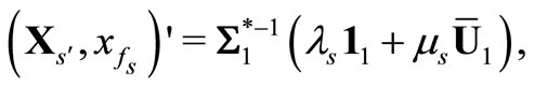
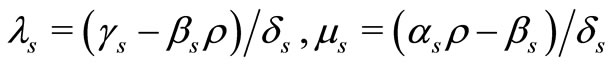
Now let  and
and . Note that
 .
.
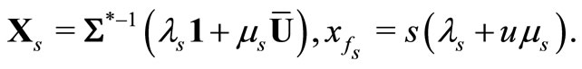
By Corollary 3.8 the primal-dual solution is
 (20)
(20)
 (21)
(21)
 (22)
(22)
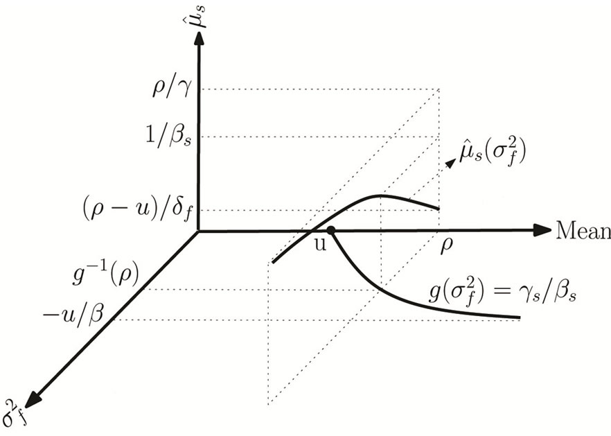
Figure 1. The continuity of  when
when .
.
 (23)
(23)
 (24)
(24)
and finally the optimal variance is
 (25)
(25)
As we know  is positive. thus the primal-dual solution and optimal variance are continuous on
 .
.
Also, it is easily seen that two parts of all of the above terms coincide at . Now the assertion holds by Theorem 3.5 and in this case, the proof is complete.
If , then for
 , part (1).(b) of Corollary 3.8 holds. Also for
 , conditions (20)-(25) hold.When β is positive the proof can be separated into two parts,
  or
or .
.
In the first case for , part 1) b) of Corollary 3.8 holds and for
 , only part 1) a) of Corollary 3.8 holds. For
 , the primal-dual solution and optimal variance are those which have stated in Equations (20)-(25). Finally in the second case for
  and
and , part 1) a) and part 1) b) of Corollary 3.8 hold, respectively. When
 , Equations (20)-(25) hold but with a change in two conditions of each equation. In all cases it is easy to investigate the continuity of primal-dual solution and optimal variance with respect to
  on the interval
 . This completes the proof.
Like Corollary 3.6 we can state the following corollary:
Corollary 3.11 Let the portfolio of Problem 3 contains a cash account  for which its rate of increments
  is uncorrelated with the total-return of the other securities. If the variance of
  converges to zero, then the primal-dual and the optimal variance of Problem 3 converges to the same values for which
  is replaced by a riskless cash account
  with the same mean total-return.
4. Co-Mean Total-Return Free Securities
In the previous section, we investigate the case in which the portfolio contains a free security. In this section we consider a portfolio with more than one free securities  which have the same mean total-return u. We call such free securities co-mean total-return or briefly co-mean free securities. Also we denote the vector weight of co-mean free securities by
and call it and its portion in the primal solution, the “free part” of the portfolio and the “free solution”, respectively. In the following, let
 for
for .
.
4.1. Portfolio with Risky and Co-Mean Free Securities
In this section we assume that the portfolio is
 where
where  and
and  are the risky and the free part of the portfolio, respectively. Let
  and
and  are the mean vector and the covariance matrix of total-returns of securities, respectively, and
  is an
is an  -column vector of ones. So the portfolio selection problem is:
Problem 2(i).
Note that Problems 2(1) an 2 are equivalent. The assumptions are the same as those stated in section 2.1, namely (A.1) and (A.3). As before, we define the following constants:

and
In the following 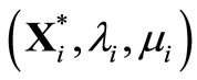 and
and  denote the primal-dual solution and the optimal variance of Problem 2(i), respectively.
Lemma 4.1. Let α, β, γ, δ and δf be the constants related to the risky part of the portfolio, then
1)
2)
3)
4)
5)
Proof. The proof is obvious.
We mention that two portfolio selection problems are equivalent, if they have the same optimal variance for any desired mean return ρ for the portfolio. Equivalently this means that their efficient frontiers coincide.
Proposition 4.2. Let . Problem 2(i) with the set of co-mean free securities

and Problem 2(j) with the set of co-mean free securities

(for j = 1 this set contains  only) are equivalent, where
 .
.
Precisely, in both problems dual solutions are identical and in primal solutions, individual weights of common securities are identical and

Proof. Considering Lemma 4.1 and the simple fact that

Theorem 2.5 shows that both problems have the same dual solutions, say  and
and , and consequently have the same optimal variance. To complete the proof let
 .
.
Then
for . Now
. Now
which is the optimal weight of the last free asset in Problem 2(j).
Proposition 4.3. Problem 2(i) and Problem 2(1) are equivalent if . Precisely, no free security appears in the primal solution of Problem 2(i), i.e.

and both problems have identical primal-dual solution.
Proof. Let . By Theorem 3.4, for
 , each free security has the following weight in the solution of Problem 2(i):
where . Now the assertion holds.
Theorem 4.4. The risky and the dual solutions, and the optimal variance of Problem 2(i) converge to that of Problem 2 when , if
, if
converges to zero. Besides, the sum of components of the free solution converges to .
.
Proof. Let  in Proposition 4.2 and construct the dummy portfolio
 where
where
 .
.
Now the assertion follows from Proposition 4.2 and Theorem 3.5.
Note. As indicated in Theorem 4.4, it is seen that
Obviously if more and more co-mean free securities with low variances are added to the portfolio, then  is more and more close to zero (this is the advantage of a set of co-mean free securities with respect to one free security). Consequently the portfolio selection problem becomes equivalent to the problem in which the set of co-mean free securities are replaced by a riskless security with that total-return in the limit sense.
4.2. Portfolio with Risky and Co-Mean Free Securities and a Guaranteed Total Loss
In this section, we investigate the effect of the presence of co-mean free securities in portfolio selection when portfolio consists of  risky securities and a total loss security. As before let
  and
and  be the risky and the free part of the portfolio, respectively. Now the portfolio is
and the problem can be stated as:
Problem 4(i).
where  is a
is a  -column vector of ones. Note that Problems 4(1) and 4 are equivalent. We display the primal-dual solution and the optimal variance of Problem
  by
by  and
and , respectively.
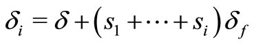
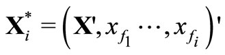
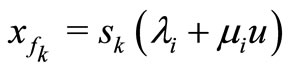
Theorem 4.5. Let . Problem 4(i) with the set of free securities
and Problem 4(j) with the set of free securities
(when , the set contains only
 ) are equivalent, where
 .
.
Precisely, in both problems dual solutions are identical and in primal solutions, individual weights of common securities are identical and
Proof. Let
 .
.
If  and
and , then by Theorem 3.7, we have
and
It can be easily seen that by Lemma 4.1 and the simple fact that
 we have
  and
and . Now the proof is straight forward by part 1) b) of Theorem 3.7. For instance in primal solution of Problem 4(j)
The claim can be proved similarly for .
.
If  and
and , the assertion follows from part 1) a) of Theorem 3.7 applied to Problems 4(i) and 4(j) and Proposition 4.2.
Theorem 4.6. Problem 4(i) and Problem 4(1) are equivalent if . Precisely, no free security appears in the primal solution of Problem 4(i), i.e.
and both problems have the identical primal-dual solution.
Proof. The case  is trivial. Let
 . Rearrange the portfolio of Problem 4(i),
  , to
, to
 .
.
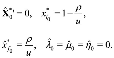
If , then by applying Proposition 3.9 for Problem 4(i), we see that the primal and dual solutions are as follows:
In this case the optimal variance is zero and this complete the proof for .
.
If , then by Proposition 3.9,
  and
and  and otherwise the primal-dual solution is identical to the primal-dual solution of Problem 2(i) when
 . On the other hand, by Theorem 4.3, the primal-dual solution is identical to the primal-dual solution of Problem 2(1). Now the assertion follows from Proposition 3.9.
Theorem 4.7. The risky, the total loss and the dual solutions, and the optimal variance of Problem 4(i) converge to that of Problem 4 when , if
, if
converges to zero. Besides, the sum of components of the free solution converges to 
Proof. Let  in Theorem 4.5 and construct the dummy portfolio
 where
where
 .
.
Now the assertion holds by Theorems 4.5 and Theorem 3.10.
Note. Theorems 3.5, 3.10, 4.4 and 4.7 state that a free security or a set of co-mean free securities which their total-returns have very low variances and the same mean with the riskless security, can be considered as a alternative for the riskless security.
REFERENCES
- H. M. Markowitz, “Portfolio Selection,” The Journal of Finance, Vol. 7, No. 1, 1952, pp. 77-91.
- J. Tobin, “Liquidity Preference as a Behavior towards Risk, Review of Economic Studies,” Vol. 25, No. 2, 1958, pp. 65-86. doi:10.2307/2296205
- R. H. Tütüncü, “A Note on Calculating the Optimal Risky Portfolio,” Finance and Stochastics, Vol. 5, No. 3, 2001, pp. 413-417. doi:10.1007/PL00013542
- R. C. Merton, “An Analytic Derivation of the Efficient Portfolio Frontier,” Journal of Financial and Quantitative Analysis, Vol. 7, No. 4, 1972, pp. 1851-1872. doi:10.2307/2329621
- R. Roll, “A Critique of the Asset Pricing Theory’s Tests. Part I. On Past and Potential Testability of the Theory,” Journal of Financial Economics, Vol. 4, No. 2, 1997, pp. 129-176. doi:10.1016/0304-405X(77)90009-5
- M. C. Steinbach, “Markowitz Revisited: Mean-Variance Models in Financial Portfolio Analysis,” Siam Review, Vol. 43, No. 1, 2011, pp. 31-85. doi:10.1137/S0036144500376650
NOTES
1Iid means independent and identically distributed.
2This notation is similar to δc in [6], when u is considered to be a return of a cash account.
3Explicitly we suppose that u is a constant.
4Explicitly we suppose that u is a constant.