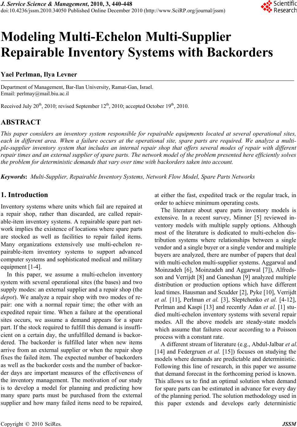J. Service Science & Management, 2010, 3, 440-448
doi:10.4236/jssm.2010.34050 Published Online December 2010 (http://www.SciRP.org/journal/jssm)
Modeling Multi-Echelon Multi-Supplier
Repairable Inventory Systems with Backorders
Yael Perlman, Ilya Levner
Department of Management, Bar-Ilan University, Ramat-Gan, Israel.
Received July 20th, 2010; revised September 12th, 2010; accepted October 19th, 2010.
ABSTRACT
This paper considers an inventory system responsible for repairable equipments located at several operational sites,
each in different area. When a failure occurs at the operational site, spare parts are required. We analyze a multi-
ple-supplier inventory system that includes an internal repair shop that offers several modes of repair with different
repair times and an external supplier of spare parts. Th e networ k model of the problem presented here efficiently solves
the problem for deterministic deman ds that vary over time with backorders taken into account.
Keywords: Multi-Supplier, Repairable Inventory Systems, Network Flow Model, Spare Parts Networks
1. Introduction
Inventory systems where units which fail are repaired at
a repair shop, rather than discarded, are called repair-
able-item inventory systems. A repairable spare part net-
work implies the existence of locations where spare parts
are stocked as well as facilities to repair failed items.
Many organizations extensively use multi-echelon re-
pairable-item inventory systems to support advanced
computer systems and sophisticated medical and military
equipment [1-4].
In this paper, we assume a multi-echelon inventory
system with several operational sites (the bases) and two
supply modes: an external supplier and a repair shop (the
depot). We analyze a repair shop with two modes of re-
pair: one with a normal repair time; the other with an
expedited repair time. When a failure at the operational
sites occurs, we assume a demand appears for a spare
part. If the stock required to fulfill this demand is insuffi-
cient on a certain day, the unfulfilled demand is backor-
dered. The backorder is fulfilled later when new items
arrive from an external supplier or when the repair shop
fixes the failed item. The expected number of backorders
as well as the backorder costs and the number of backor-
der days are important measures of the effectiveness of
the inventory management. The motivation of our study
is to develop a model for planning and predicting how
many spare parts must be purchased from the external
supplier and how many failed items need to be repaired,
at either the fast, expedited track or the regular track, in
order to achieve minimum operating costs.
The literature about spare parts inventory models is
extensive. In a recent survey, Minner [5] reviewed in-
ventory models with multiple supply options. Although
most of the literature is dedicated to multi-echelon dis-
tribution systems where relationships between a single
vendor and a single buyer or a single vendor and multiple
buyers are analyzed, there are number of papers that deal
with multi-echelon multi-supplier systems. Aggarwal and
Moinzadeh [6], Moinzadeh and Aggarwal [7]), Alfreds-
son and Verrijdt [8] and Ganeshan [9] analyzed multiple
distribution or production options which have different
lead times. Hausman and Scudder [2], Pyke [10], Verrijdt
et al. [11], Perlman et al. [3], Sleptchenko et al. [4-12],
Perlman and Kaspi [13] and recently Adan et al. [1] stu-
died multi-echelon inventory systems with several repair
modes. All the above models are steady-state models
which assume that failures occur according to a Poisson
process with a constant rate.
A different stream of literature (e.g., Abdul-Jalbar et al.
[14] and Federgruen et al. [15]) focuses on studying the
models where demands are predictable and deterministic.
Following this line of research, in this paper we assume
that demand forecast in the forthcoming period is known.
This allows us to find an optimal solution when demand
for spare parts can be estimated in advance for every day
of the planning period. The solution methodology used in
this paper extends and develops early deterministic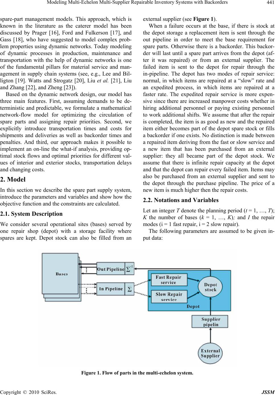

Modeling Multi-Echelon Multi-Supplier Repairable Inventory Systems with Backorders 441
spare-part management models. This approach, which is
known in the literature as the caterer model has been
discussed by Prager [16], Ford and Fulkerson [17], and
Gass [18], who have suggested to model complex prob-
lem properties using dynamic networks. Today modeling
of dynamic processes in production, maintenance and
transportation with the help of dynamic networks is one
of the fundamental pillars for material service and man-
agement in supply chain systems (see, e.g., Lee and Bil-
ligton [19]. Watts and Strogatz [20], Liu et al. [21], Liu
and Zhang [22], and Zheng [23]).
Based on the dynamic network design, our model has
three main features. First, assuming demands to be de-
terministic and predictable, we formulate a mathematical
network-flow model for optimizing the circulation of
spare parts and assigning repair priorities. Second, we
explicitly introduce transportation times and costs for
shipments and deliveries as well as backorder times and
penalties. And third, our approach makes it possible to
implement an on-line the what-if analysis, providing op-
timal stock flows and optimal priorities for different val-
ues of interior and exterior stocks, transportation delays
and changing costs.
2. Model
In this section we describe the spare part supply system,
introduce the parameters and variables and show how the
objective function and the constraints are calculated.
2.1. System Description
We consider several operational sites (bases) served by
one repair shop (depot) with a storage facility where
spares are kept. Depot stock can also be filled from an
external supplier (see Figure 1).
When a failure occurs at the base, if there is stock at
the depot storage a replacement item is sent through the
out pipeline in order to meet the base requirement for
spare parts. Otherwise there is a backorder. This backor-
der will last until a spare part arrives from the depot (af-
ter it was repaired) or from an external supplier. The
failed item is sent to the depot for repair through the
in-pipeline. The depot has two modes of repair service:
normal, in which items are repaired at a “slow” rate and
an expedited process, in which items are repaired at a
faster rate. The expedited repair service is more expen-
sive since there are increased manpower costs whether in
hiring additional personnel or paying existing personnel
to work additional shifts. We assume that after the repair
is completed, the item is as good as new and the repaired
item either becomes part of the depot spare stock or fills
a backorder if one exists. No distinction is made between
a repaired item deriving from the fast or slow service and
a new item that has been purchased from an external
supplier: they all became part of the depot stock. We
assume that there is infinite repair capacity at the depot
and that the depot can repair every failed item. Items may
also be purchased from an external supplier and sent to
the depot through the purchase pipeline. The price of a
new item is much higher then the repair costs.
2.2. Notations and Variables
Let an integer T denote the planning period (t = 1, …, T);
K the number of bases (k = 1, …, K); and I the repair
modes (i = 1 fast repair, i = 2 slow repair).
The following parameters are assumed to be given in-
put data:
Figure 1. Flow of parts in the multi-echelon system.

Modeling Multi-Echelon Multi-Supplier Repairable Inventory Systems with Backorders 442
Rt (k): the required number of good items on day t in base
k
Ft (k): the entering flow of failed items on day t in base k
n: shipping time at the in pipeline
m: shipping time at the out pipeline
l: lead time from external supplier to the depot
p: repair time at slow repair service
q: repair time at fast repair service

qp
c: cost charged for transporting a unit item
e: cost charged for buying a new unit item
i: cost charged for repairing a unit item at depot ser-
vices i
a

12
ea a
h: inventory holding cost per unit item
d: cost charged for distributing a unit item
b: penalty cost for per unit backordered
We introduce the following (integer) variables:
0 qt(k): the number of failed items sent from base k
on day t

0 lt(k): the number of failed items left unsent at base
k on day t

0 Qt(k): the flow of failed items that arrived at the
depot from base k on day t

0 DSt : the depot stock of good items on day t 
0 xt: the number of items entering the fast repair ser-
vice at the depot on day t

0 yt: the number of items entering the slow repair
service at the depot on day t

0 Xt: the number of items repaired at the fast repair
service in the depot on day t

0 Yt: the number of items repaired at the slow repair
service in the depot on day t

0 ut: the number of items ordered from external sup-
plier on day t

0 Ut: the number of items that arrived at the depot
stock from supplier on day t

0 St: the number of good items sent from the depot
on day t

0 zt: the number of good items sent from depot to
base k on day t

0 Zt(k): the number of good items that arrived to base
k on day t

0 BOt(k)i: the number of backordered demands at
base k on day t

2.3. Mathematical Modeling Framework
Our objective is to minimize the total cost of transporting,
distributing, repairing, holding, purchasing and backor-
dering of items during the planning period:
Minimize:
     

12
tt tt
tk tk
tt ttt
ttt ttk
cqkzkdQkzk
axayhDSeubBOk
 
 
 
  (1)
The constraints are as follows:
S. t.
Ft(k) + lt-1(k) = qt(k) + l
t(k) (2)
Qt (k) = qt-n(k) (3)
Σk Q
t(k) = xt + y t (4)
Xt = xt-q (5)
Yt = yt-p (6)
Ut = ut-l (7)
Xt + Yt + Ut + DSt-1 = DSt + S
t (8)
SIt = Σk zt(k) (9)
Zt+m(k) = zt(k) (10)
Zt(k) + BOt(k) = R
t(k) + BOt-1(k) (11)
Constraint (2) is the balance of failed items at the base.
The number of failed items qt(k) sent from base k to the
in-pipeline on day t plus the number of failed items lt(k)
left unsent at base k on day t must be equal to the flow
(the number) of all failed items Ft(k) entering base k on
day t plus the number of failed items lt-1(k) left unsent in
base k on day t-1.
Constraint (3, 10) is the transportation of failed (re-
spectively good) items at the in-pipeline (out-pipeline).
The flow of failed items leaving base k to the depot on
day t-n arrives through the in-pipeline at the depot on day
t. Where the number of good items entering the
out-pipeline for base k on day t-m arrives at base k on
day t.
Constraint (4) is the integrating and distributing of
failed items from different bases. The number of failed
items entering the depot from all the bases on day t is
distributed between the fast and slow repair services on
day t.
Constraints (5-6) are the repair of failed items and
their “conversion” to good ones. The number of failed
items xt (respectively, yt) entering the fast (respectively,
slow) service on day t-q (respectively, t-p) repair service
is converted into the same number of good items on day
t.
Constraint (7) is the purchasing of a new item from an
external supplier. The number ut-l of new items ordered
from an external supplier on day t-l that arrives at the
depot on day t.
Constraint (8) is the balance of depot stock. The num-
ber of repaired items from both the fast repair service and
the slow repair service on day t, plus the number Ut of
new items that arrived from the external supplier on day t,
plus DSt-1 the depot stock on day t-1 is equal to DSt the
depot stock on day t plus the number of items St sent
from the depot to the out-pipeline on day t.
Constraint (9) is the distribution of good items from

Modeling Multi-Echelon Multi-Supplier Repairable Inventory Systems with Backorders 443
the depot between different out-pipelines to the different
bases. The total number of sent items from the depot on
day t is equal to the sum items zt(k) sent into the
out-pipeline for base k =1, …, K.
Constraint (11) is the balance of good items at the base.
The number of good items Zt(k) transported to base k
from the depot through the out-pipeline on day t plus
BOt(k) the number of backordered demands at base k on
day t is equal to the required number of good items Rt on
day t plus the number of backordered demands at base k
on day t-1.
2.4. Network Flow Model
Figure 2 presents a network formulation of this problem
for a special case of two bases. The time parameters are
given in Table 1.
2.5 Numerical Example for the Network
Flow Model
There are two bases and the planning period is 6 days.
The requirements for good items is equal to the num-
ber of failed items thus Rt (k) = Ft (k) where: R (1) = (5-9)
and R (2) = (6,6,7,10,8,5). There is an initial stock of 15
spares at the depot. Table 1 presents the time parameters
while Table 2 gives the cost parameters. The optimal
result given in Table 3 is presented in Figure 3 as a
network flow.
3. Experimental Results
3.1. Parameters
We present experimental results from an air force envi-
ronment where airplanes are operating from three bases.
Each base has 20 airplanes. The planning horizon is a
16-day wartime scenario where the planner knows the
number of sorties scheduled for each base on each day
during the planning horizon. This allows planners to pre-
dict the utilization rate of the airplane service for each
day for each base as well as the number of flight hours
that the fleet will make at each base on each day.
Figure 2. Network flow model.

Modeling Multi-Echelon Multi-Supplier Repairable Inventory Systems with Backorders 444
The unit we analyze is the airplane’s air data computer.
A computer backorder grounds an airplane. Given the
MTBF (mean time between failures) of the computer and
the flight hours planned for each aircraft, which varies
from day to day depending on the war scenario, the
number of failed computers for each day at each base can
be predicted. Table 4 presents the number of failed
computers. It is assumed that the requirement for each
day equals the number of failed items. The input pa-
rameters are listed in Table 5.
3.2. Numerical Results
It is assumed that all parameters are known (see Table 5).
The “what-if” analysis is conducted in order to study the
parameters: depot initial stock, backorder penalty cost,
fast service repair time and fast service cost. We list the
optimal results and discuss their implications (see Tables
6-7).
Table 1. The time parameters.
Shipping-time at the in-pipeline n = 1 days
Shipping time at the out-pipeline m = 1 day
Lead time from external supplier
to depot l = 1 day
Repair time at slow repair service p = 3 days
Repair time at fast repair service q = 2 days
Table 2. Cost data.
Distribution cost d = 0 $
Transportation cost c = 0.05 $
Fast repair cost a1 =15$
Slow repair cost a2 = 10$
Purchase cost e = 25$
Inventory holding cost h = 0. 5$
Backorder penalty cost b= 40$
Table 3. Optimal planning.
Day
Number of
failed items to
enter fast repair
service
Number of
failed items to
enter slow repair
service
Number of items to
purchase from
external supplier
1 0 0 22
2 9 2 18
3 12 0 6
Table 4. Number of failed computers-prediction.
Base 1 Base 2 Base 3
Day 1 4 5 2
Day 2 4 4 3
Day 3 6 3 8
Day 4 8 2 2
Day 5 7 2 9
Day 6 6 4 4
Day 7 6 4 3
Day 8 5 4 4
Day 9 4 6 8
Day 10 2 6 9
Day 11 2 6 7
Day 12 2 7 9
Day 13 8 6 6
Day 14 8 7 8
Day 15 8 6 2
Day 16 7 5 2
Table 5. Input parameters.
Shipping time at the in-pipeline n = 1 days
Shipping time at the out-pipeline m = 1 day
Lead time from external supplier
to depot l = 1 day
Repair time at slow repair service p = 5 days
Repair time at fast repair service q = 3 days
Distribution cost D = 0 $
Transportation cost c = 0.05 $
Fast repair cost A1 =15$
Slow repair cost A2 = 10$
Purchase cost e = 100$
Inventory holding cost h = 0. 5$
Backorder penalty cost B= 20$
Initial depot stock DS0=30 parts
From Table 6 it can be seen that occasionally there are
backorders. On the first day there are backorders since it
akes a minimum of one day for spares to arrive from the t

Modeling Multi-Echelon Multi-Supplier Repairable Inventory Systems with Backorders 445
Table 6. Optimal flow of items at the base.
Failed items left unsent at
base k Failed items sent to the depot from base k Good items sent from the depot to base k Backordered demands at base k
Day l1 l2 l3 q1 q2 q3 z1 z2 z3 BO1 BO2 BO3
1 0 0 2 4 5 0 8 9 5 4 5 2
2 0 0 0 4 4 5 6 3 8 0 0 0
3 0 0 0 6 3 8 8 2 2 0 0 0
4 0 0 0 8 2 2 7 2 9 0 0 0
5 0 1 0 7 1 9 6 4 4 0 0 0
6 0 0 0 6 5 4 6 4 3 0 0 0
7 0 0 0 6 4 3 5 4 4 0 0 0
8 0 0 0 5 4 4 4 6 8 0 0 0
9 0 0 0 4 6 8 2 6 9 0 0 0
10 0 0 0 2 6 9 2 6 7 0 0 0
11 2 0 0 0 6 7 2 7 9 0 0 0
12 4 7 9 0 0 0 8 6 6 0 0 0
13 12 13 15 0 0 0 8 7 6 0 0 0
14 20 20 23 0 0 0 8 5 4 0 0 2
15 28 26 25 0 0 0 7 6 2 0 1 0
16 35 31 27 0 0 0 0 0 0 0 0 0
Table 7. Optimal flow of items at the depot.
Failed items entering/exiting the fast
repair service Failed items entering/exiting the slow repair service
Good items or-
dered/arriving
from external supplier
Depot stock (good
items)
Day
x X y Y U U DS0 = 30
1 0 0 0 0 9 0 8
2 5 0 4 0 12 9 0
3 0 0 13 0 18 12 0
4 9 0 8 0 9 18 0
5 5 5 7 0 13 9 0
6 9 0 8 0 0 13 0
7 8 9 7 4 0 0 0
8 10 5 3 13 0 0 0
9 13 9 0 8 0 0 0
10 18 8 0 7 0 0 0
11 17 10 0 8 0 0 0
12 15 13 0 7 0 0 0
13 0 18 0 3 0 0 0
14 0 17 0 0 0 0 0
15 0 15 0 0 0 0 0
16 0 0 0 0 0 0 0

Modeling Multi-Echelon Multi-Supplier Repairable Inventory Systems with Backorders 446
depot (the out-pipeline equals 1 day). On days 14 and 15
respectively. This optimal result is obtained due to the
cost parameters. For example, on day 13 there are only
21 repaired items from both fast and slow services, while
the total number of orders at day 14 is 23. Thus there is a
backorder of two parts. The optimal result is to maintain
this backorder since the backorder penalty cost at this
stage is $20 while the cost of a new item (the only way to
fill this backorder) is much higher at $100. When the
backorder penalty cost is increased, the number of back-
orders is reduced to zero (see the what-if analysis below).
The total number of new items purchased from an exter-
nal supplier is 61 parts. The total number of items re-
paired at the fast service is 109 parts and at the slow ser-
vice 50. This mixture is a result of both cost parameters
and delay time parameters. Although fast repair service is
more expensive, more items are sent to the fast service
due to the need to quickly supply repaired items to fill
the orders at the bases. In addition, the ratio between the
cost of fast and slow repair equals 1:5. Increasing this
ratio reduces the total number of items repaired in the
fast service and increases the total number of items re-
paired at the slow service (see what-if analysis below)
3.3. What-If Analysis
3.3.1. Initial Depot Stock
Initial depot stock is the amount of stock that the air
force purchases in advance and holds at the depot. There
is a tradeoff between holding a high initial depot stock at
the start of the planning horizon and making a mix of
purchases and repairs along the planning horizon. The
procurement price of this stock is often paid in advance
and entails extra inventory holding costs at the depot. We
study the implication of a change in initial depot stock
level. In Table 8, the results show what happens when
the initial depot stocks vary from 30 spares to 110. When
the initial stock rises from 30 to 91 spares, there is a re-
duction in spares purchased from the external supplier by
the same amount. There is no change in the number of
backorders and the time they occur. When the initial de-
pot stock exceeds 91 spares there is no need to purchase
parts from an external supplier. When there is a high lev-
el of initial stock, there is a change in the optimal mix of
repairs. Specifically, more parts are repaired at the slow
service and there are zero backorders. Thus from the
point of depot stocks equaling 91, the slow service is
used more than the fast service, since this service is
cheaper and with high depot stock there is no need for a
short repair time.
3.3.2 Backorder Penalty Cost
Estimating the backorder penalty cost is based on the
availability target set by the air force. High backorder
cost results in a small number of backorders, and vice
versa. We study the effect of changing backorder costs
from $20 to $70 and consider backorders that are non-
trivial, that is, backorders that occur from the second day
on (see Table 9).
Table 8. Changes in initial depot stock.
Initial
depot
stock
Total number of parts
repaired at fast service Total number of parts repaired at slow service
Total number of parts pur-
chased from external sup-
plier
Total number of
backorders
(non-trivial)
Objective
function
value
30 109 50 61 3 8539
50 109 50 41 3 6554
70 109 50 21 3 4584
90 109 50 1 3 2628
100 61 89 0 0 2164
110 27 113 0 0 1925
Table 9. Changes in backorder penalty cost.
Backorder
penalty cost Total number of backorders Numb e r of d ay s with backorders Total number of purchases Total number of fast repairs Total number of slow repairs Objective func- tion value
20 3 2 61 109 50 8539
30 3 2 61 109 50 8679
40 1 1 62 104 54 8804
50 1 1 62 104 54 8924
60 1 1 62 104 54 9044
70 0 0 63 99 58 9159

Modeling Multi-Echelon Multi-Supplier Repairable Inventory Systems with Backorders 447
Table 10. Changes in fast repair time.
Fast service
repair time Total number of purchases Total number of fast repairs Total number of slow repairs Total number of backorders Number of days with backorders Objective func- tion value
3 61 109 50 3 2 8539
2 43 146 31 7 2 7185
1 20 195 5 23 4 5680
Table 11. Changes in fast repair service cost.
Fast repair ser-
vice Cost
Total number of parts repaired
at fast service
Total number of parts repaired at
slow service
Total number of parts purchased from
external supplier
15 109 50 61
20 104 54 62
40 25 117 78
Analyzing the results reveals that when backorder pe-
nalty costs increase, both the total number of backorders
and the number of days with backorders decreases grad-
ually and slowly. When the backorder penalty cost equals
70, there are zero backorders. The changes in backorder
costs causes minor changes in the mix of repaired and
purchased parts along the planning horizon. The total
number of items repaired at the fast repair service is re-
duced by a small amount while the total number of both
new items and of repaired items at the slow repair in-
creases by a small amount.
3.3.3. Repair Time at the Depot Fast Service
The repair time is effected by repair resources such as
manpower and equipment that the air force allocates.
Hiring extra, better qualified manpower may shorten the
repair time. In studying the impact of a shorter repair
time at the fast service, we reduced the fast repair time to
2 and 1 days (see Table 10). As a result, more parts are
sent to repair at the fast repair service since it has become
more attractive. For example, when the fast repair time
equals the lead-time from an external supplier (both
equal one day), and since the cost of the fast repair is
much cheaper than the purchase cost, almost all the spare
parts that are needed come from the fast repair service.
The fact that there are more backorders when the repair
time decreases is an interesting result that emerges be-
cause the depot can only repair the items that failed. Thus
there are sometimes delays in getting repaired items from
the fast repair service, as opposed to the external supplier
who can fulfill any amount that has been ordered.
3.3.4. Cost of the Fast Repair Service
The ratio of the fast and slow repair services can be set
by the air force as a tool to motivate and control the us-
age of the two repair modes. Note that these prices are
also called transfer-prices. Table 11 presents the results
of changing fast service costs from $15 to $ 40.
4. Conclusions
In this paper we studied a repairable–item multi-echelon
inventory system with multiple supply alternatives: an
external supplier and fast and slow repair services. We
considered the demand for spare part as a deterministic
demand that can be predicted for a specified horizon.
During the planning horizon, demand varies dramatically
over time due to a change in the utilization rate of the
parts. Our network flow model allows planning the opti-
mal number of items that need to be repaired at each re-
pair mode and the optimal number of new items that
need to be purchased from an external supplier. Our
model facilitates what-if analysis with different cost pa-
rameters and delay time parameters. This analysis is
useful for practical real-life situations in order to plan
and control the spare parts supply chain.
REFERENCES
[1] I. J. B. F. Adan, A. Sleptchenko and G. J. J. A. N. van
Houtum, “Reducing Costs of Spare Parts Supply Systems
via Static Sriorities,” Asia-Pacific Journal of Operational
Research, Vol. 26, No. 4, 2009, pp. 559-585.
[2] W. Hausman and G. Scudder, “Priority Scheduling Rules
for Repairable Inventory Systems,” Management Science,
Vol. 28, No. 11, 1982, pp. 1215-1232.
[3] Y. Perlman, A. Mehrez and M .Kaspi, “Setting Expedit-
ing Repair Policy in a Multi-Echelon Repairable-Item In-
ventory System with Limited Repair Capacity,” Journal
of the Operational Research Society, Vol. 52, 2001, pp.
198-209.
[4] A. Sleptchenko, M. C. van der Heijden and A. van Harten,
“Using Repair Priorities to Reduce Stock Investment in
Spare Part Networks,” European Journal of Operations

Modeling Multi-Echelon Multi-Supplier Repairable Inventory Systems with Backorders 448
Research, Vol. 163, 2005, pp. 733-750.
[5] S. Minner, “Multiple-supplier Inventory Models in Sup-
ply Chain Management: A Review,” International Jour-
nal of Production Economics, Vol. 81, 2003, pp. 265-279.
[6] P. K. Aggarwal and K. Moinzadeh, “Order Expedition in
Multi-echelon Production/Distribution Systems,” IIE
Transaction, Vol. 2, No. 2, 1994, pp. 86-96.
[7] K. Moinzadeh and P. K. Aggarwal, “An Information Base
multi-Echelon Inventory System with Emergency Ord-
ers,” Operations Research, Vol. 45, 1997, pp. 694-701.
[8] P. Alfredsson and J. Verrijdt, “Modeling Emergency Su-
pply Flexibility in a Two Echelon Inventory System,”
Management Science, Vol. 45, No. 10, 1999, pp. 1416-
1431.
[9] R. Ganeshan, “Managing Supply Chain Inventories: A
multiple Retailer, One Warehouse, Multiple Supplier
Model,” International Journal of Production Economics,
Vol. 59, 1999, pp. 341-354.
[10] D. F. Pyke, “Priority Repair and Dispatch Policies for
Repairable-Item Logistics Systems,” Naval Research Lo-
gistics, Vol. 37, 1990, pp. 1-30.
[11] J. Verrijdt, I. Adan and T. de Kok, “A Tradeoff between
Repair and Inventory Investment,” IIE Transactions, Vol.
30, 1998, pp. 119-132.
[12] A. Sleptchenko, M. C. van der Heijden and A. van Harten,
“Effect of Finite Repair Capacity in Multi-Echelon, Mul-
ti-Indenture Service Part Supply Systems,” International
Journal of Production Economics, Vol. 79, No. 2, 2002,
pp. 209-230.
[13] Y. Perlman and M. Kaspi, “Centralized Decision of In-
ternal Transfer-Prices with Congestion Externalities for
Two Modes of Repair with Limited Repair Capacity,”
Journal of the Operational Research Society, Vol. 58, No.
9, 2007, pp. 1178-1184.
[14] B. Abdul-Jalbar, J. M. Gutierrez and J. Sicilia, “Single
Cycle Policies for the One-Warehouse N-Retailer Inven-
tory/Distribution System,” Omega, Vol. 34, No. 5, 2006,
pp. 196-208.
[15] A. Federgruen, J. Meissner and M. Tzur, “Progressive
Interval Heuristics for Multi-Item Capacitated Lot Sizing
Problems,” Operations Research, Vol. 55, No. 3, 2007,
pp. 490-502.
[16] W. Prager, “On the Caterer Problem,” Management Sci-
ence, Vol. 3, 1956, pp. 16-23.
[17] L. R Ford and D. R. Fulkerson, “Flows in Networks,”
Princeton University Press, 1962.
[18] S. I. Gass, “Linear Programming: Methods and Applica-
tions,” Dover Publications, 2003.
[19] H. Lee and C. Billigton, “Material Management in De-
centralized Supply Chains,” Operations Research, Vol.
41, 1993, pp. 837-845.
[20] D. J. Watts and S.H. Strogatz, “Collective Dynamics of
‘Small World’ Networks,” Nature, Vol. 393, No. 6684,
1998, pp. 440-442.
[21] X. Liu, C. Wang, X. Luo and D. Wang, “A Model and
Algorithm for Outsourcing Planning,” Proceedings IEEE
International Conference on E-Business Engineering
ICEBE’05, Beijing, 2005, pp. 1-4.
[22] X. Liu and J. Zhang, “A Capacitated Production Planning
with Outsourcing: A General Model and Its Algorithm,”
Lecture Notes in Computer Science, Vol. 4113, 2006, pp.
997-1002.
[23] J. Zheng, “A Modeling Framework for the Planning of
Strategic Supply Chains Viewed from Complex Net-
work,” Journal of Service Science & Management, Vol. 2,
No. 2, 2009, pp. 129-138.