Volatility Forecasting of Market Demand as Aids for Planning Manufacturing Activities
384
tainty over future market conditions, decide on its pro-
duction schedule? To keep on top of demand, a company
has to avoid shortages on one hand and too much invent-
tory on the other. This means that forecasting is a key
issue, whether the company builds its own products in its
own factories or outsources its production. Short of being
able to control market, demand planning and scheduling
manufacturing operations depend on an ability to predict
what will be the market demand and how it will fluctuate
during the execution of plans generally frozen over a
certain horizon.
Forecasting by extrapolating historical data (linear re-
gression, simple and double exponential smoothing, de-
composition of time-series in trends, cyclical variations
and randomness …..) [2] is a technique over-described in
textbooks and research papers. It is straightforward to
apply and could be justified in the postwar “fordist” era.
Today volatility is the key feature of the global economy:
the fluttering of a butterfly in Bejing can trigger a tor-
nado in Cuba.
The irreversibility of a decision and the possibility of
delaying its implementation are two important charac-
teristics when converting forecasts into scheduled
courses of action. A manufacturing company with an
opportunity to schedule production is holding an “op-
tion” analogous to a financial call option on a common
stock - it has the right and not the obligation, at some
future time of its choosing, to make an expenditure
(manufacturing a batch of products) and receive a
revenue (the proceeds of their sale) [3]. When such a
company decides on a schedule, it exercises, or “kills”,
its option to manufacture. It gives up the possibility of
waiting for complementary information to arrive that
might affect the desirability or timing of the expendi-
ture incurred by the scheduled production versus the
market value of the manufactured products, value
which fluctuates stochastically. The option can be “in
the money” meaning that when it is exercised it would
yield a positive payoff. It is said to be “out of the
money” if exercising yields a negative payoff. It cannot
disinvest2 that is get back the money already spent,
should market conditions change adversely.
An investment project, such as manufacturing a batch
of products, can be made more valuable if it gives the
manufacturer the option to expand when economic con-
ditions become favorable. That option to expand in the
future clearly has a value. The higher the volatility of the
underlying asset - the market demand - the higher value
is given to the option - the market value of the batch of
products manufactured to sell. Economists assume that
the selling price of a product depends on the market de-
mand expressed in terms of quantity of products so that
the proceeds of a sale increase along with market de-
mand.
3. Market Volatility and the Associated
Risks
3.1. Volatility
Volatility is the relative rate at which market demand
moves up and down. It is found by calculating, over a
period of time, the standard deviation of daily, weekly or
monthly change in market demand. The time intervals
considered are impelled to be chosen by the behavior of
market demand. If it moves up and down rapidly over
short periods of time, it is highly volatile. On the con-
trary if market demand is almost never changed it has
low volatility.
The risk that the scheduler of manufacturing activities
is exposed to, is based on the potential for the volatility
of the underlying market demand or the market’s percep-
tion of that volatility to change. It is generally assumed
that uncertainty in the future depends on the time span.
The longer the time interval, the greater is uncertainty
about the situation by the end of this time interval and, as
a consequence, the volatility of a variable z under con-
sideration. To match with this commonly accepted belief,
the time-dependent probability density function of the
variable z at a fixed time, when normally distributed, is
[4]
2
1
,exp
2
2.
z
fzt t
t
(1)
The mean value of at any time is
zt
,0Ezt
and the variance of at time is
zt
t t,zVar
.
In many contexts of business life changes in the values
of a variable are not measured in absolute terms but as
increments with respect to its values, that is in relative
terms. That is why volatility is calculated as the variance
of a log function representing the values of a variable at
different times.
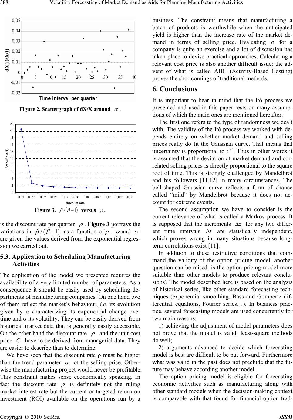
Denoting the market demand as for the time
interval i, the volatility of this variable is defined as the
standard deviation of the function
Di
/ 1Di Diln
with 1in
.
3.2. Wiener Process
A Markov process is a particular type of stochastic proc-
ess where only the present value of a variable is relevant
for predicting the future. The past history of the variable
is supposed to be embedded in its present value. Predic-
tions for the future are uncertain and must be expressed
in terms of probability distribution. If the weak form of
market efficiency were not true, analysts could make
above-average returns on stocks by interpreting the cha-
rts of the past history.
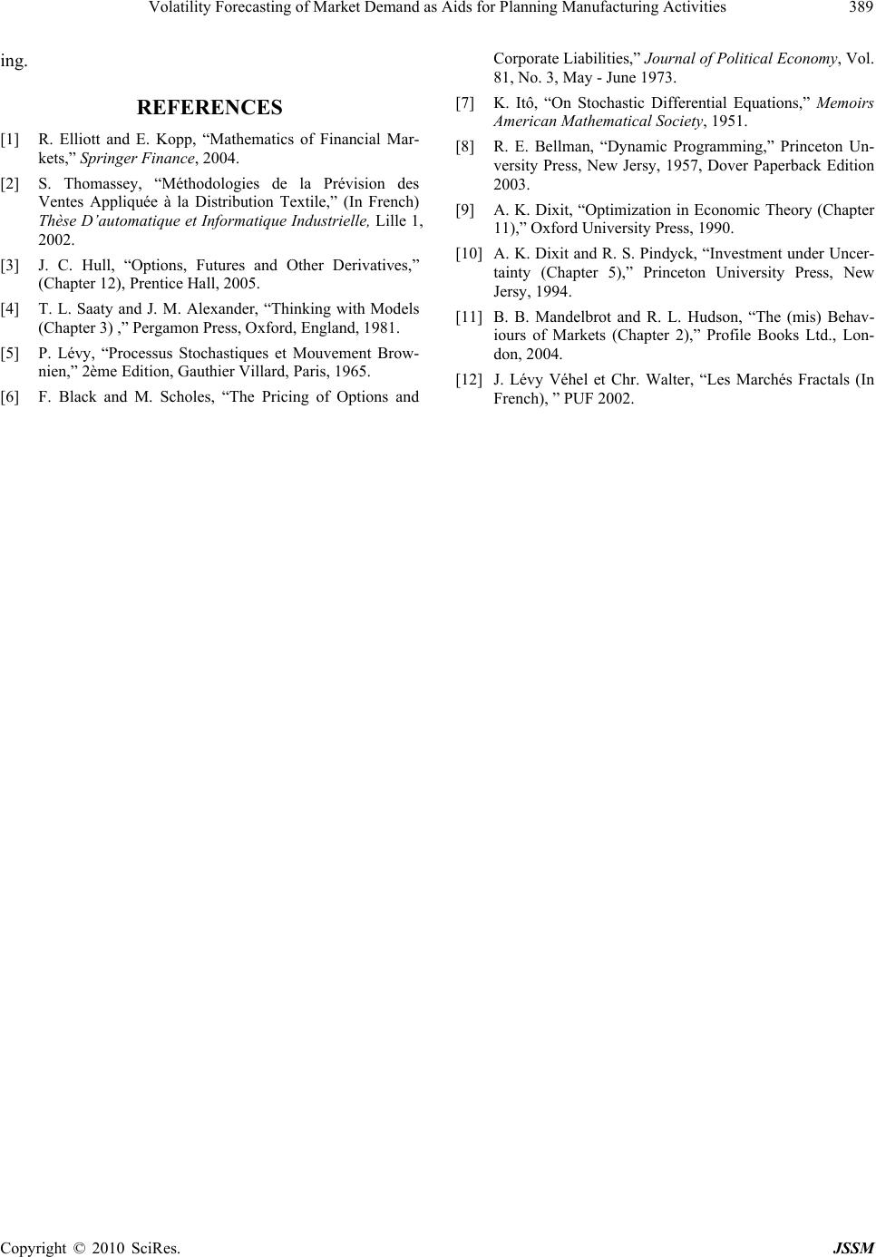
Copyright © 2010 SciRes. JSSM