Int. J. Communications, Network and System Sciences, 2010, 3, 907-915
doi:10.4236/ijcns.2010.312124 Published Online December 2010 (http://www.SciRP.org/journal/ijcns)
Extraction of Signals Buried in Noise: Non-Ergodic
Processes
Nourédine Yahya Bey
UFR des Sciences, Département de Physique, Université François Rabelais, Tours, France
Received April 15, 2010; revised August 19, 2010; accepted October 2 , 20 10
Abstract
In this paper, we propose extraction of signals buried in non-ergodic processes. It is shown that the proposed
method extracts signals defined in a non-ergodic framework without averaging or smoothing in the direct
time or frequency domain. Extraction is achieved independently of the nature of noise, correlated or not with
the signal, colored or white, Gaussian or not, and locations of its spectral extent. Performances of the pro-
posed extraction method and comparative results with other methods are demonstrated via experimental
Doppler velocimetry measurements.
Keywords: Buried Signals, Stationary Non-Ergodic Processes, Spectral Analy sis, White Noise, Colored
Noise, Correlated Noise, Doppler Velocimetry
1. Introduction
Quality of signal information in different areas of science
is degraded by encountered various natures of noises.
This degradation may take different forms and evolves to
observations where the time-averaged correlation func-
tion of a process is different from the ensemble-averaged
function [1,2]. Non-linear filtering and their correspond-
ing asymptotic stability are gen erally proposed to handle
such processes [3-5].
In situations where signals are totally buried in noise
and for which no a-priori information is available, er-
godic hypothesis cannot be validated. Moreover, none of
the above methods is suitable for extraction of such bur-
ied signals. In real world situations, non-ergodic proc-
esses in which a desired signal is buried may occur as
shown by Doppler velocimetry measurements [6-11]
used in this work.
It is crucial to notice that by the terms extraction of
signals, we mean extraction of clean spectra of buried
signals in noise and by buried signals, we mean signals
defined for low or extreme low signal-to-noise ratio. In
[12,13], we proposed two equivalent extraction methods,
called respectively “modified frequency extent denoising
(MFED)” and “constant frequency extent denoising
(CFED)”. For easy reference, let us recall that the fre-
quency extent is the interval


0, e
f
where e
f
is the
sampling frequency of the buried continuous-time signal
to be extracted. The first procedure (MFED) is based on
modifying the sampling frequency and the second one
(CFED) is suited to a collection of available sample
noisy processes for which the sampling frequency is
constant. Clearly, CFED offers implementation simplic-
ity since in most applications, signals are defined for a
constant sampling frequency. Proposed extraction does
not use any a-priori information on the signal to be ex-
tracted, works without averaging or smoothing in the
direct time or dual frequency space, and it is achieved
independently of the nature of noise (colored or white,
Gaussian or not) and locations of its spectral extent.
Extraction methods in [12,13] are based on the theory
of ergodic stationary processes. Extension of these re-
sults to extraction of signals correlated with noise in
which they are buried are reported in [14]. We have
shown that extraction of signals correlated with noise is
achieved without averaging and independently of the
nature of noise (correlated or not, correlated or not with
the signal, colored or white, Gaussian or not) and loca-
tions of its spectral extent.
In this work, we extend results of one of the afore-
mentioned extraction methods (CFED), to a more gen-
eral case where ergodic hypothesis, given experimental
conditions, cannot be validated, which is a fact and an
issue.

908 N. Y. BEY
In Section 2, we recall principal definitions and results
of the CFED extraction method since this method offers
implementation simplicity as mentioned above. In Sec-
tion 3, expression of extracted spectra of buried signals
from non-ergodic processes is derived without any sort
of averaging or smoothing in the time or frequency do-
main and without assuming the signal uncorrelated with
noise. Extraction performances and comparative results
with other methods [15-18] are discussed and illustrated
in Section 4. It is shown that CFED extracts the Doppler
mean frequency from experimental Doppler velocimetry
measurements for which ergodic hypothesis is not vali-
dated or satisfied.
2. Fundamentals [12,13]
In this section, we recall some principal results reported
in [12,13].
2.1. Signal Representation
Let us consider a finite observation of

T
zt


zt, a
process containing a band-limited signal buried in
zero-mean wide sense stationary noise , in the in-
terval of length with m. The process

bt

T1
ax
Tf ≫


t
T
z,
available at the output of a low-pass filter of cut-off fre-
quency max
f
, is given by ,
  


,0,
=0, otherwise,
TT
T
bt sttT
zt  

 (1)
where and

T
bt

T
s
t represent respectively the
additive noise (white or co lored) and the signal observed
in the time interval of length .
T
By considering the ins tants =
ne
tn where mx f2
ea
f
f
is the sampling frequency, we can define the discrete-
time process with .
()
N
zn =e NTf
2.2. The Sample Power Spectral Density (SPSD)
[12]
Given , we can form the
estimate,
  
0,1,,1
NN N
zz zN

   
2
,, =1DFT,
e
ffTTz nN


(2)
where DFT denotes Discrete Fourier Transform
of . Here the estimate


N
zn

N
zn

,,
e
f
fT depends on
the frequency,
f
, the sampling frequency, e
f
, and the
length of the observation interv al, . T
It is crucial to notice that (2) is not a power spectral
density in the usual sense. In [12], (2) is defined as the
“Sample” power spectral density or the sample spectrum
of the process . In the following, we recall for
easy reference the CFED extraction method.

N
zn
2.3. CFED Extraction Method
Here, we have a collection of

realizations of dura-
tion of a noisy process so that the length of the total
observation interval is
TT

. These

realizations de-
noted where


p
T
zt =0p, ,1

 are now con-
catenated, i.e.,
 
1()
=0
=
p
TT
p
zt ztpT



. (3)
2.3.1. Sampl e Spec trum of Noise
We found that the sample spectrum of noise obtained by
Fourier transformation of (3) is given by [12],
  

1
=0
,, =,,,
ep
p
ffTfpT fT

 

e
(4)
where




,,
e
fp TfT   are translated copies of
the original sample spectrum of noise whose components
are spaced with the mutual distance 1/ on the fre-
quency axis. T
It is crucial to notice that

p

 in (4) are reduction
factors defined by,

1
=0 =1.
p
p



 (5)
For the sake of simplicity and without loss of general-
ity, we let,

=0,,1,=1.
p
p

   (6)
Notice that a justification of (6) is found in [14]. Fac-
tors


p

 reduce indifferently translated copies the
original sample spectrum of noise independently of their
nature (white or colored, Gaussian or not) and act indif-
ferently at all frequencies.
2.3.2. Spectral Distributi o n
Spectral lines of each copy of the original sample spec-
trum of noise




,,
e
f
pTfT   of noise are sepa-
rated by the mutual distance . As these copies are
shifted by 1/T


1T

with respect to each other (see (4)),
the resulted sample spectrum

,,
e

f
fT

 will exhibit
spectral lines separated by the mutual distance


1T

.
Hence original spectral lines of noise separated by the
mutual distance 1T are now distributed in new

frequency locations created in each frequency interval of
length 1T.
On the other hand, the spectrum of the signal


T
s
t
as given by the transformation of concatenated realiza-
tions (3), is specified by

,,
e
f
fT

. Since

zeros
are distributed in

frequency locations created in each
interval of length 1T (see [12]) then,

N. Y. BEY
909

e

,, =,,.
e
f
fT ffT   (7) depicted by (10), is given by,






*
*
,, =,,,,
,, ,,
,,,,,
ee
ee
ee


e
f
fTffT ffT
Sff Tff T
Sff Tff T

 
 
 



(11)
2.3.3. Extraction Procedure
Extraction of the sample spectrum of the buried signal is
obtained by decimation. This decimation by the factor

is applied in the frequency domain to the Fourier
transformation of (3). The signal-to-noise ratio


of the
decimated spectrum written as a function of the sig-
nal-to-noise ratio of the original spectrum is given
by, 
where


,,
e
Sff T

and

,,
e

f
fT

 represent the
amplitude spectra of respectively the signal and noise.
Here


*
x
 is the complex conjugate of


x
 and


,,
e
f
fT

 is the sample spectrum of

concate-
nated realizations of noise.

.

  (8) Now, let us find the optimal form under which expres-
sion of the CFED sample spectrum is written only as a
function of the sample spectrum of the signal and noise
independently of any correlation between the signal and
noise and without averaging in the time or frequency
domain.
We have shown in [12] that increasing

increases
the signal-to-noise ratio of the original noisy spec-
trum 

,,
e

f
fT in which the desired signal is buried.
Moreover, the variance of sample spectral estimates of
noise tends to zero as

increases.
3.1.1. Sampl e Spec trum of Noise
3. Non-Ergodic Processes Expression of the sample spectrum of noise of a
non-ergodic process is obtained by using the above ex-
pression (4) derived under the ergodic assumption. In
(4), one finds translated copies of the original sample
spectrum of noise, denoted in the ergodic case by




,,
e
f
pTfT  , of each realization or sample
process for =0,,1p


.
Here, we extend above results obtained for ergodic sta-
tionary processes to processes for which ergodic hy-
pothesis cannot be validated or satisfied. We consider
therefore that we have a collection of

sequences
whose probability density functions that describe noise
affecting them are different from sequence to an other
one. This means that any sample process can be put un-
der the form,
Now, in the non-ergodic framework, as depicted by
(10), it is crucial to notice that we have

realizations
defined for different and unknown noise distributions. As
in (10) the index (p) identifies each noise distribution,
here, we introduce the index (p) in order to identify their
corresponding

original and different sample spectra.
We can therefore rewrite (4) by identifying translated
copies of original sample spectra of noise by their corre-
sponding upper script


p (for =0,,1p


) as
follows,

 


=
p
TTT
tstbt  ,
p
(9)
where

T
s
t

t
is the signal defined above and
is the additive noise specified for the realization (p).
Moreover, probability density functions describing
for


p
T
bt


p
T
b=0,,1p

 are assumed unknown.
Clearly the process from which samples are
taken is stationary and not ergodic. Covariances of the
 p
T


t

sample processes are dependent on the
sample process (see p. 89 of [19], for the definition
of non-ergodic processes). For implementation simplicity,
we use hereafter the CFED method, recalled above,
where those


p
Tt


p

samples of a non-ergodic process are
concatenated, i.e.,
  
1()
=0
,, =,,,
p
epp
p

e
f
fT ffT

 

 (12)
where,

 

() ()
,, =,,.
pp
pe e
f
fTfpT fT   (13)

1
() ()
=0
()= .
p
TT T
p
tstpT btpT




 



p


(10) 3 . 1.2. Decimated CFED Sample Spectrum
The decimated N-point sample spectrum applied to


,,
e
f
fT

, as depicted by (11), yields (14).


is the

-decimation applied to

. where



3.1. CFED Sample Spectrum Notice that since the power spectral density of the sig-
nal is assumed constant in collected

sequences then
decimated sample spectrum of the signal yields the same
The sample spectrum of the process of duration T

, as
 



**
,, =,,,,
,,,,,,,, ,
eee
eee e
ff Tff Tff T
SffT ffTSffTffT



 
 





 (14)

N. Y. BEY
910
result as (7).
On the other hand, since we have

translated and
different copies of original sample spectra of noise then
decimation in the frequency domain yields a spectrum in
which contribute coefficients of those

copies of
original spectra of noise. This means that the coeffi-
cients of the decimated spectrum described by (12) are
those of the translated copies
N

 
,,
pe
f
pTfT  
for =0, ,1p


. Notice that this applies also to the
amplitude spectra of noise

,,
e

f
fT


. This means
that by setting


=1
p


, the decimated sample
spectrum of noise in (14) becomes,
   


1()
=0
(0)( 1)
,, =,,
=1,, ;,,,
p
ep
p
e
e
f
fT fpTfT
ffT




 




 







 (15)
where the set of the copies is given by


0
,,





1



,,
pe
f
pTfT   for =0, ,1p


(0)
,,;
e
ffT 
.
Since Fourier coefficients of
are those of the translated copies
noise variance

( 1)
,,





01
,,



 then the
2


of is given
by,
 

01
; ,,T





,
,,
e
ff
222
min max
<<

 (16)
where 2
min

and 2
max

are respectively the smallest and
the greatest noise variances contained in the collection of

sequences.
It is crucial to notice that (16) is at the heart of this work.
According to (16), we can assume, for the sake of sim-
plicity and without loss of generality, that the decimated
sample spectrum of noise
approaches the average sample spectra of the translated
copies of noise. Under this assumption,
justified by (16), we can write the variance of the deci-
mated sample spectrum of noise
 

0
,,; ,,
e
ffT




 

0
,,; ,,
e
ffT

as follows,


1
1
22
=0 =0
==1N,
p
k
kp
c


 


 (17)
where

p
k
cfor =0 1kN

 and =0 1p



,, 
are Fou-
rier coefficients of the translated copies
 
01 


.
Now, according to (17), the sample spectrum



0
,,; ,,
e
ffT



1 written as a function of its
Fourier coefficients, yields,


1
(0)( 1)
=0
,,; ,,=,
N
ek
k

f
fTcf kT





 (18)

1
1

1

0
,,







where
 


01
=
kkk
cc c



 represents the average
of coefficients of translated copies

0
,,


1

. Notice
that the ergodic case [12,13] can be obtained from (18)
by setting
 
01
==
kk
cc


.
By using (7) and (15), the decimated sample spectrum
of the process, as given by (14), is therefore given by,









(0)( 1)
*(0)( 1)*(0)( 1)
,,=,,1,,; ,,
,,,,; ,,,,,,; ,,,
ee e
eee e
DffT ffTffT
S ffTffTSffTffT




 


 




(19)
where decimated power spectrum of noise written as a function of its amplitude spectra yields,





(0)1(0)( 1)*(0)( 1)
,,;,,=,,;,,,,;,,.
eee
ffTffT ffT

 


 
 (20)
3.2. Optimal CFED Sample Spectrum
Let us in the following find a condition under which the
decimated sample spectrum as depicted by (19) can be
written without rectangular terms (cross-products). The
optimal form is that for which the sample spectrum is
described only as function of the spectra of the signal
and noise.
Let k

be Fourier coefficients of the amplitude
spectrum of the signal and let

,,
e
SffT

k

be
Fourier coefficients of the amplitude noise spectrum
. Since,
 
0
; ,,





,, =ffT


ff 
S
1

e
,,
eT


*
,, ,,,
ee
ffTSffT (21)
then according to (20) and (21), we have,

*
*
=
=,
kkk
kkk
c


(22)
where k c is defined in (18).
By using (22), the sample spectrum, as given by (19),
yields therefore explicitly,
 



(0) 1
1**
=0
,,=1,,;,,
.
ee
N
kkk kk
k
ff TffT
fkT



 






 




(23)
3.2.1. The Optimal Reduction Factor
In the following, we derive the optimal reduction factor
or the optimal number of concatenated sample processes

N. Y. BEY
911

under which contribution of th e cross-produ cts in (19)
is made negligible. Coefficients of the last right-hand
side of (23) can be put u nder the form,

*
**=1
kk
kkkkk kkk
.


 





 








(24)
Let

*
=
kkkkk


   and note that,
11
k, k

  (25)
where k

rewritten as a function of k

and k

yields,
*
2
k
kk
kk k
.







 (26)
By setting

*
=
kk
ck


, (26) becomes,
*
2
kk k
kk k
c 
.






 (27)
Now, let us find the condition that defines the mini-
mum v a l u e o f

under which (27) is smaller than unity,
i.e.,
2
k
k
c

≪1. (28)
We propose to find

as a function of the mean sig-
nal-to-noise ratio of the

collection of different proc-
esses. Let us define the mean signal-to-noise ratio of the
collected

sample processes by,
2
=,
s
p


where
s
p represents the mean power of the signal
and



22 2
01 
=



 is the mean variance of
noise of the collected

sample processes. Here

p
2

is noise variance of the sample process


p (for
=0, 1p,

).
The mean signal-to-noise ratio can be written under
the form,
2
=
=,
s
k
kc
p
I
cI




 (29)
where k

and k c are arbitrary chosen coefficients and,
1
=0,
1
=0,
=1
=1/ ,
s
k
ssk
cq
qqk
I
k
I
cc












 (30)
where and 

represent respectively the number
of components of the signal and noise.
It is easy to see that I

is bounded by,


,minmax,
sk sk
kI



   (31)
where


min
s
k

 and

max

s
k

 denote respec-
tively the minimum and the maximum values of the set
formed by
s
k

, for and = 0,1,,1sk

.
Since k

is an arbitrary chosen coefficient and ac-
cording to (31), we can consider that,
,=kI

.

 (32)
Similarly, =
c
I

. The signal-to-noise ratio, as de-
picted by (29), becom es,
=.
k
k
c



(33)
Now, the expression (28) is satisfied if,
4.


≫

(34)
For a useful interpretation of (34), we express the op-
timal reduction factor

only as a function of the mean
signal-to-noise ratio

. By setting


min =4


 ,
one finds that since <1 two conditions have to be
considered : 41

 and 4 1. This gives,
min
min
1
41,1<
1
41,.








(35)
As min

 ≫ in accordance with (34), then by
choosing

exceeding the upper bound of the variation
interval of min

, or,
1
>, 
 (36)
the condition (28) is fulfilled.
Here (36) depicts the optimal reduction factor

as a
function of the mean signal-to-noise ratio  of the col-
lection of

non-ergodic sample processes. This opti-
mal reduction factor represents therefore the number of
concatenated sample processes.
3.2.2. Optimal CFED Spectrum
According to (36), (2 4) yields,
**
>1 ,.
kkkkk k





  (37)
By using (37), ( 2 3) bec omes,

 

(0)( 1)
>1 ,, ,, ,
1,,;,,.
ee
e
f
fT ffT
ffT







 



(38)
This yields,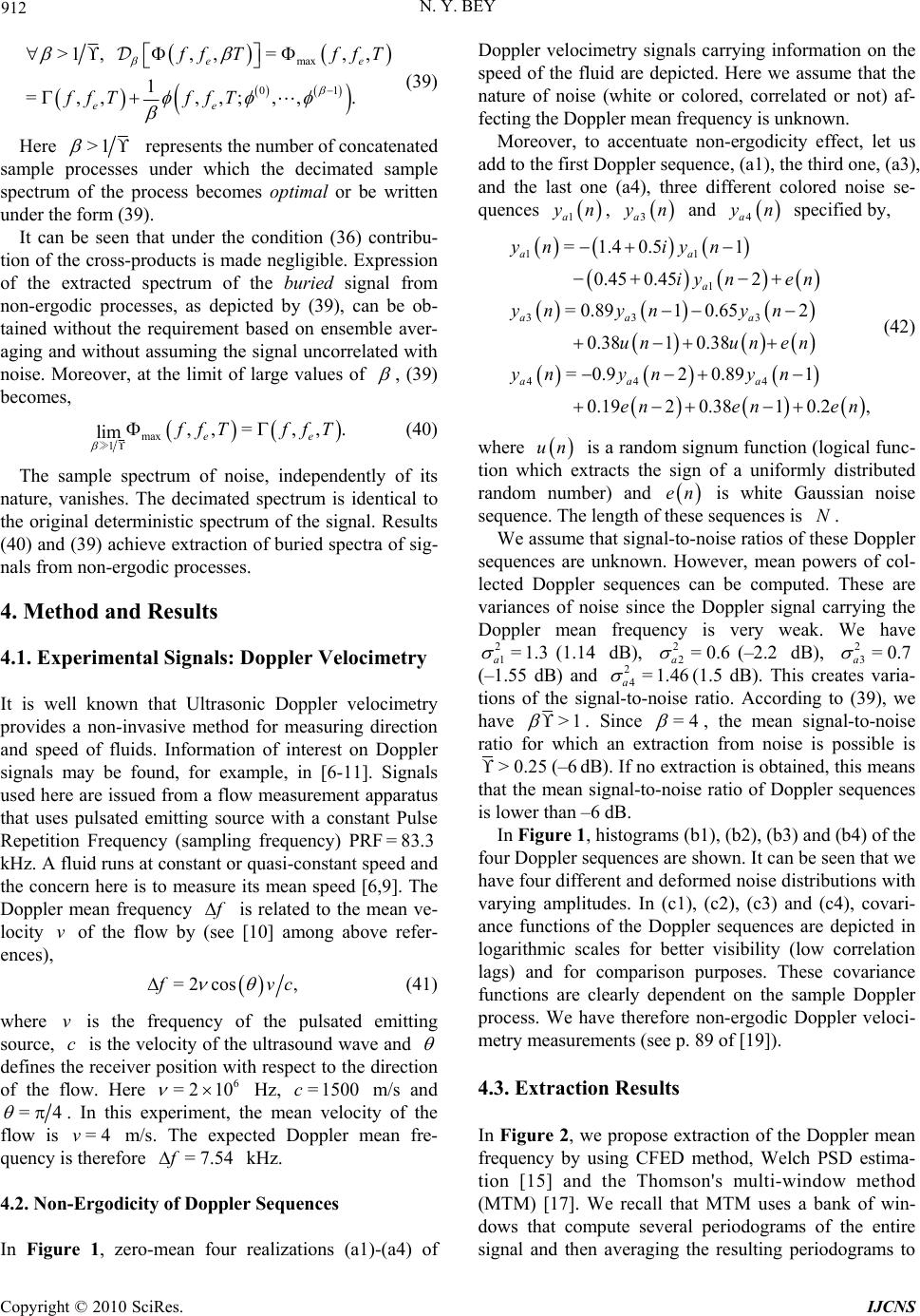

912 N. Y. BEY





max
01
>1 ,, ,=, ,
1
=,,,,;,, .
e
ee 
e
f
fT ffT
ffTffT






  

 

(39)
Here >1   represents the number of concatenated
sample processes under which the decimated sample
spectrum of the process becomes optimal or be written
under the form (39).
It can be seen that under the condition (36) contribu-
tion of the cross-pro ducts is made negligible. Expression
of the extracted spectrum of the buried signal from
non-ergodic processes, as depicted by (39), can be ob-
tained without the requirement based on ensemble aver-
aging and without assuming the signal uncorrelated with
noise. Moreover, at the limit of large values of

, (39)
becomes,

max
1,, =,,.
lim e

e
f
fT ffT
  ≫ (40)
The sample spectrum of noise, independently of its
nature, vanishes. The decimated spectrum is identical to
the original deterministic spectrum of the signal. Results
(40) and (39) achieve extraction of buried spectra of sig-
nals from non-ergodic processes.
4. Method and Results
4.1. Experimental Signals: Doppler Velocimetry
It is well known that Ultrasonic Doppler velocimetry
provides a non-invasive method for measuring direction
and speed of fluids. Information of interest on Doppler
signals may be found, for example, in [6-11]. Signals
used here are issued from a flow measurement apparatus
that uses pulsated emitting source with a constant Pulse
Repetition Frequency (sampling frequency) PRF =8
kHz. A fluid runs at constant or quasi-constant speed and
the concern here is to measure its mean speed [6,9]. The
Doppler mean frequency
3.3
f
 is related to the mean ve-
locity of the flow by (see [10] among above refer-
ences),
v


=2 cos,
f
vc   (41)
where is the frequency of the pulsated emitting
source, is the velocity of the ultrasound wave and
v
c

defines the receiver position with respect to the direction
of the flow. Here Hz, m/s and
6
=2 10  =1500c
=4

. In this experiment, the mean velocity of the
flow is m/s. The expected Doppler mean fre-
quency is therefore kHz.
=4v=7.54f
4.2. Non-Ergodicity of Doppl er Sequence s
In Figure 1, zero-mean four realizations (a1)-(a4) of
Doppler velocimetry signals carrying information on the
speed of the fluid are depicted. Here we assume that the
nature of noise (white or colored, correlated or not) af-
fecting the Doppler mean frequency is unknown.
Moreover, to accentuate non-ergodicity effect, let us
add to the first Doppler sequence, (a1), the third one, (a3),
and the last one (a4), three different colored noise se-
quences


1a
y
n,


3a
y
n and

4a
y
n specified by,



 


 

 
11
1
33 3
44 4
=1.40.51
0.45 0.452
= 0.8910.652
0.3810.38
= 0.920.891
0.1920.3810.2,
aa
a
aa a
aa a
yn iyn
iy nen
yn ynyn
unun en
yn ynyn
enen en
 
 
 
 
 


(42)
where


un is a random signum function (logical func-
tion which extracts the sign of a uniformly distributed
random number) and


en is white Gaussian noise
sequence. The length of these sequences is . N
We assume that signal-to-noise ratios of these Doppler
sequences are unknown. However, mean powers of col-
lected Doppler sequences can be computed. These are
variances of noise since the Doppler signal carrying the
Doppler mean frequency is very weak. We have
(1.14 dB), (–2.2 dB),
(–1.55 dB) and a(1.5 dB). This creates varia-
tions of the signal-to-noise ratio. According to (39), we
have
21=1.3
a

22=0.6
a

=1.46
23=0.7
a

24

>1  . Since =4

, the mean signal-to-noise
ratio for which an extraction from noise is possible is
>0.25 (–6 dB). If no extraction is obtained, this means
that the mean signal-to-noise ratio of Doppler sequences
is lower than –6 dB.
In Figure 1, histograms (b1), (b2), (b3) and (b4) of the
four Doppler sequences are shown. It can be seen that we
have four different and deformed noise distributions with
varying amplitudes. In (c1), (c2), (c3) and (c4), covari-
ance functions of the Doppler sequences are depicted in
logarithmic scales for better visibility (low correlation
lags) and for comparison purposes. These covariance
functions are clearly dependent on the sample Doppler
process. We have therefore non-ergodic Doppler veloci-
metry measurements (see p. 89 of [19]).
4.3. Extraction Results
In Figure 2, we propose extraction of the Doppler mean
frequency by using CFED method, Welch PSD estima-
tion [15] and the Thomson's multi-window method
(MTM) [17]. We recall that MTM uses a bank of win-
dows that compute several periodograms of the entire
ignal and then averaging the resulting periodograms to s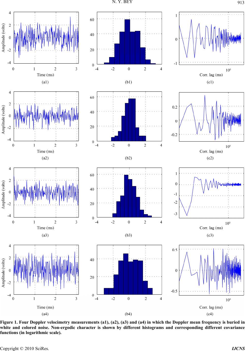

N. Y. BEY
913
Figure 1. Four Doppler velocimetry measurements (a1), (a2), (a3) and (a4) in which the Doppler mean frequency is buried in
white and colored noise. Non-ergodic character is shown by different histograms and corresponding different covariance
functions (in logarithmic scale).

914 N. Y. BEY
Figure 2. CFED spectrum and its decimated version are shown in (a) and (b) where the Doppler frequency is extracted
(7.55 kHz). Comparison with Welch PSD and the Thomson's multitaper method is provided in (c) and (d).
construct a spectral estimate. In order to minimize the
bias and variance in each window, theses windows are
chosen orthogonal. Optimal windows that satisfy these
requirements are Slepian sequences or discrete prolate
spheroidal sequences [18].
Now, these four realizations

are concate-
nated and the obtained process, as given by (10), is ana-
lyzed by the above methods. The spectrum of CFED
concatenated realizations and its decimated version
are respectively shown in Figures 2(a) and (b).
The frequency of the depicted spectral line (Doppler
mean frequency) is


=4 

=4 

f
 = 7.55 kHz. The obtained va ria-
tion with respect to the above expected Doppler fre-
quency is 0.13%. The Welch periodogram estimation
shows however a widened peak located at 7.4 kHz with a
weak signal-to-noise ratio whereas the MTM method
depicts with a much weaker signal-to-noise ratio a spec-
tral line far from the expected Doppler mean frequency.
It can be seen that independently of the nature of noise
(white or colored, correlated or not) affecting experi-
mental signals and variation of the signal-to-noise ratio,
the Doppler mean frequency is clearly extracted by
CFED from non-ergodic process with an excellent sig-
nal-to-noise ratio without any averaging in the time or

N. Y. BEY
915
frequency domain and without using any a-priori infor-
mation on the signal (Doppler mean frequency) and the
nature of noise in which the signal is buried.
5. Conclusions
In this work, extraction theory of signals buried in
non-ergodic processes is proposed. We have shown that
no a-priori information on the signal to be extracted is
used and no averaging in the direct time or frequency
domain is performed. Observed results on experimental
Doppler velocimetry measurements buried in non-ergodic
processes show that extraction of the Doppler mean fre-
quency is achieved independently of the nature of noise,
correlated or not with the signal, colored or white, Gaus-
sian or not, and locations of its spectral extent. Observed
results are in accordance with theoretical predictions.
6. Acknowledgements
The author wishes to express his thanks to anonymous
reviewers for their constructive suggestions.
7. References
[1] J. L. Starck and F. Murtagh, “Astronomical Image and
Data Analysis,” Springer Verlag Inc., New York, 2006.
[2] P. N. Pusey and W. va n Megen, “Dynamic Light Scatter-
ing by Non-Ergodic Media,” Royal Signals and Radar
Establishment, Physica A, Vol. 157, No. 2, 1989, pp.
705-741.
[3] A. Budhiraja and D. Ocone, “Exponential Stability in
Discrete Time Filtering for Non-Ergodic Signals,” Sto-
chastic Processes and Their Applications, Vol. 82, No. 2,
1999, pp. 245-257.
[4] N. Oudjane and S. Rubenthaler, “Stability and Uniform
Particle Approximation of Nonlinear Filters in Case of
Non Ergodic Signals,” Stochastic Analysis and Applica-
tions, Vol. 23, No. 3, 2005, pp. 421-448.
[5] G. Storvik, “Particle Filters for State Space Models with
the Presence of Unknown Static Parameters,” IEEE
Transactions on Signal Processing, Vol. 50, No. 2, 2002,
pp. 281-289.
[6] W. D. Barber, J. W. Eberhard and S. G. Kaar, “A New
Time-Domain Technique for Velocity Measurements
Using Doppler Ultrasound,” IEEE Transactions on Bio-
medical Engineering, Vol. BME-32, No. 3, 1985, pp. 213-
229.
[7] P. J. Vaitkus and R. S. C. Cobbold, “A Comparative
Study and Assessment of Doppler Ultrasound Spectral
Estimation Techniques Part I: Estimation Methods,” Ul-
trasound in Medicine and Biology, Vol. 14, No. 8, 1988,
pp. 661-672.
[8] P. J. Vaitkus, R. S. C. Cobbold and K. W. Johnston, “A
Comparative Study and Assessment of Doppler Ultra-
sound Spectral Estimation Techniques Part II: Method
and Results,” Ultrasound in Medicine and Biology, Vol.
14, No. 8, 1988, pp. 673-688.
[9] D. H. Evans, W. N. MacDicken, R. Skidmore and J. P.
Woodcock, “Summary of the Basic Physics of Doppler
Ultrasound,” Doppler Ultrasound, Physics Instrumenta-
tion and Clinical Applications, Wiley, Chichester, 1989.
[10] J. Arendt, “Estimation of Blood Velocities Using Ultra-
sound,” Cambridge University Press, Cambridge, 1996.
[11] A. Herment and J. F. Giovanelli, “An Adaptive Approach
to Computing the Spectrum and Mean Frequency OD
Doppler Signal,” Ultrasonic Imaging, Vol. 17, No. 1, 1995,
pp. 1-26.
[12] N. Y. Bey, “Extraction of Signals Buried in Noise, Part I:
Fundamentals,” Signal Processing, Vol. 86, No. 9, 2006,
pp. 2464-2478.
[13] N. Y. Bey, “Extraction of Signals Buried in Noise, Part II:
Experimental Results,” Signal Processing, Vol. 86, No.
10, 2006, pp. 2994-3011.
[14] N. Y. Bey, “Extraction of Buried Signals in Noise: Cor-
related Processes,” International Journal of Communica-
tions, Network and System Sciences, Vol. 3, No. 11, 2010,
pp. 855-862.
[15] P. D. Welch, “The Use of Fast Fourier Transform for the
Estimation of Power Spectra: A Method Based on Time
Averaging over Short, Modified Periodograms,” IEEE
Transactions on Audio and Electroacoustics, Vol. AU-15,
1967, pp. 70-73.
[16] S. M. Kay and S. L. Marple, “Spectrum Analysis—A
Modern Perspective,” Proceedings of IEEE, Vol. 69, No.
11, 1981, pp. 1380-1419.
[17] D. J. Thomson, “Spectrum Estimation and Harmonic
Analysis,” Proceedings of the IEEE, Vol. 70, No. 9, 1982,
pp. 1055-1096.
[18] Y. Xu, S. Haykin and R. J. Racine, “Multiple Window
Time-Frequency Distribution and Coherence of EEG Us-
ing Slepian Sequences and Hermite Functions,” IEEE
Transactions on Biomedical Engineering, Vol. 46, No. 7,
1999, pp. 861-866.
[19] J. S. Bendat, “Measurement and Analysis of Random
Data,” John Wiley and Sons Inc., Hoboken, 1966.