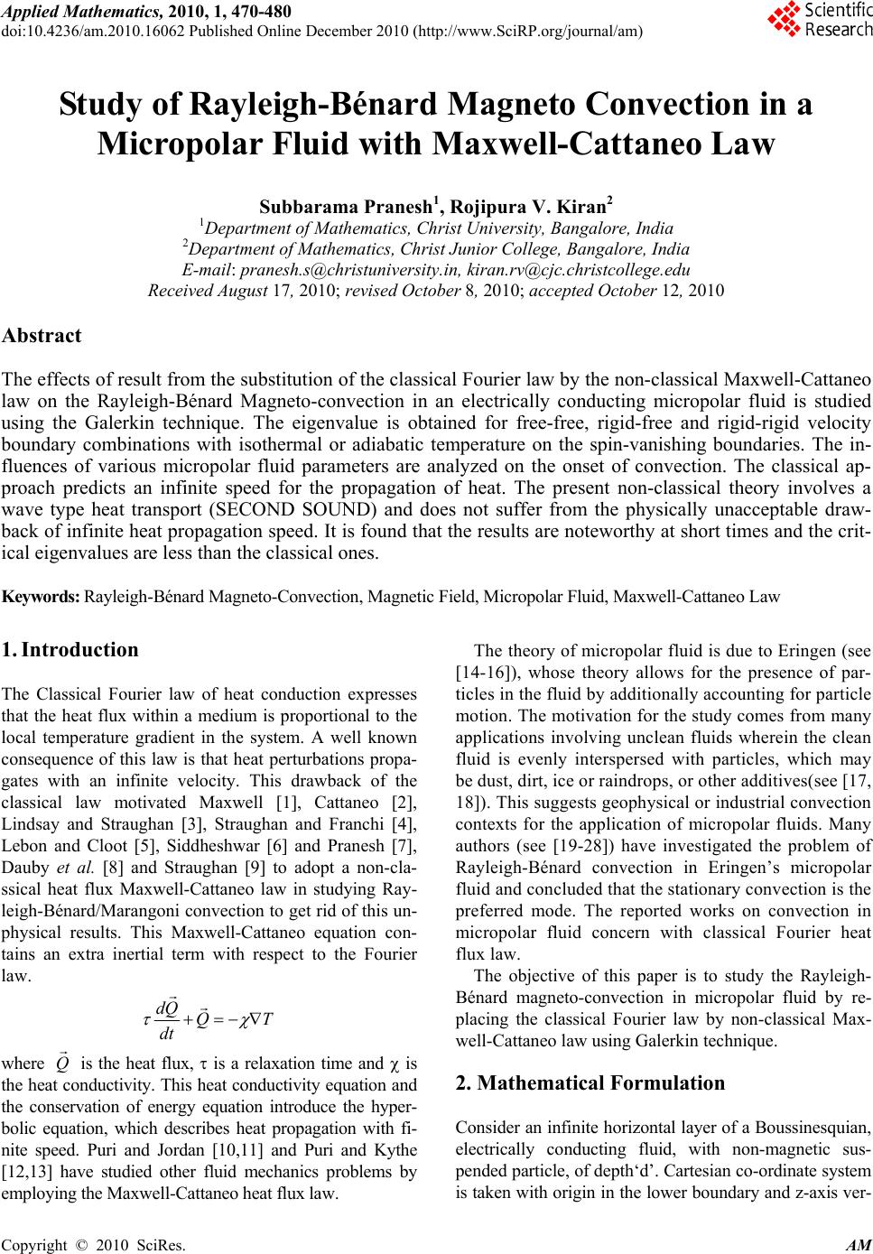Applied Mathematics, 2010, 1, 470-480
doi:10.4236/am.2010.16062 Published Online December 2010 (http://www.SciRP.org/journal/am)
Study of Rayleigh-Bénard Magneto Convection in a
Micropolar Fluid with Maxwell-Cattaneo Law
Subbarama Pranesh1, Rojipura V. Kiran2
1Department of Mathematics, Christ University, Bangalore, India
2Department of Mathematics, Christ Junior College, Bangalore, India
Received August 17, 2010; revised October 8, 2010; accepted October 12, 2010
Abstract
The effects of result from the substitution of the classical Fourier law by the non-classical Maxwell-Cattaneo
law on the Rayleigh-Bénard Magneto-convection in an electrically conducting micropolar fluid is studied
using the Galerkin technique. The eigenvalue is obtained for free-free, rigid-free and rigid-rigid velocity
boundary combinations with isothermal or adiabatic temperature on the spin-vanishing boundaries. The in-
fluences of various micropolar fluid parameters are analyzed on the onset of convection. The classical ap-
proach predicts an infinite speed for the propagation of heat. The present non-classical theory involves a
wave type heat transport (SECOND SOUND) and does not suffer from the physically unacceptable draw-
back of infinite heat propagation speed. It is found that the results are noteworthy at short times and the crit-
ical eigenvalues are less than the classical ones.
Keywords: Rayleigh-Bénard Magneto-Convection, Magnetic Field, Micropolar Fluid, Maxwell-Cattaneo Law
1. Introduction
The Classical Fourier law of heat conduction expresses
that the heat flux within a medium is proportional to the
local temperature gradient in the system. A well known
consequence of this law is that heat perturbations propa-
gates with an infinite velocity. This drawback of the
classical law motivated Maxwell [1], Cattaneo [2],
Lindsay and Straughan [3], Straughan and Franchi [4],
Lebon and Cloot [5], Siddheshwar [6] and Pranesh [7],
Dauby et al. [8] and Straughan [9] to adopt a non-cla-
ssical heat flux Maxwell-Cattaneo law in studying Ray-
leigh-Bénard/Marangoni convection to get rid of this un-
physical results. This Maxwell-Cattaneo equation con-
tains an extra inertial term with respect to the Fourier
law.
TQ
dt
Qd 



where Q

is the heat flux,  is a relaxation time and  is
the heat conductivity. This heat conductivity equation and
the conservation of energy equation introduce the hyper-
bolic equation, which describes heat propagation with fi-
nite speed. Puri and Jordan [10,11] and Puri and Kythe
[12,13] have studied other fluid mechanics problems by
employing the Maxwell-Cattaneo heat flux law.
The theory of micropolar fluid is due to Eringen (see
[14-16]), whose theory allows for the presence of par-
ticles in the fluid by additionally accounting for particle
motion. The motivation for the study comes from many
applications involving unclean fluids wherein the clean
fluid is evenly interspersed with particles, which may
be dust, dirt, ice or raindrops, or other additives(see [17,
18]). This suggests geophysical or industrial convection
contexts for the application of micropolar fluids. Many
authors (see [19-28]) have investigated the problem of
Rayleigh-Bénard convection in Eringen’s micropolar
fluid and concluded that the stationary convection is the
preferred mode. The reported works on convection in
micropolar fluid concern with classical Fourier heat
flux law.
The objective of this paper is to study the Rayleigh-
Bénard magneto-convection in micropolar fluid by re-
placing the classical Fourier law by non-classical Max-
well-Cattaneo law using Galerkin technique.
2. Mathematical Formulation
Consider an infinite horizontal layer of a Boussinesquian,
electrically conducting fluid, with non-magnetic sus-
pended particle, of depth‘d’. Cartesian co-ordinate system
is taken with origin in the lower boundary and z-axis ver-

S. PRANESH ET AL.
471
tically upwards. Let T be the temperature difference
between the upper and lower boundaries. (See Figure 1)
The governing equations for the Rayleigh-Bénard situa-
tion in a Boussinesquian fluid with suspended particles are
Continuity equation:
.0,q
 (1)
Conservation of linear momentum:



2
ˆ
.
2.,
o
m
qqqP gk
t
qHH

 


 


 

 


  (2)
Conservation of angular momentum:
 


2
..
2,
oIq
t
q


 



 



 

 


  (3)
Conservation of energy:
..,
ov
TqTQ
tC



 




 (4)
Maxwell-Cattaneo heat flux law:
.
1,QQQT
 

 



 (5)
Magnetic induction equation:


2
.. ,
m
HqHHq H
t

  

 

(6)
Equation of state:

1
oo
TT  



. (7)
where q
 is the velocity,


is the spin,
T
is the tem-
perature,
P
is the hydromagnetic pressure,
H

is the
magnetic field,

is the density, o

is the density of
the fluid at reference temperature o
TT , g is the acce-
leration due to gravity,

is the coupling viscosity co-
efficient or vortex viscosity,

is the shear kinematic
viscosity coefficient,
I
is the moment of inertia,


and 
are the bulk and shear spin viscosity coefficient,

T
0
+

T
T
0
O
X
Z = d
Z = 0
Micropol a r Fluid
Z
Figure 1. Schematic diagram of the Rayleigh-Bénard situa-
tion for micropolar fluid.
is the micropolar heat conduction coefficient, v C is the
specific heat,

is the thermal conductivity,

is the
coefficient of thermal expansion,
mm
m


1
 is the
magnetic viscosity :( m

electrical conductivity andm

:
magnetic permeability), 1
1,
2qQ
  
is the heat
flux vector and

is the constant relation time.
The basic state of the fluid being quiescent is de-
scribed by
 
  
ˆ
0, 0,,
,,
0, 0,,
bb bo
bb
bb
qHHk
PPz z
QQzTTz



 

 








(8)
Equations (2), (4), (5) and (7) in the basic state speci-
fied by “(8)” respectively become

2
2
ˆ,0,
,
1,
0.
bb
o
b
b
bo bo
b
dP dQ
gk
dz dz
dT
Qdz
TT
dT
dz


 

 


 











(9)
Equations (1), (3) and (6) are identically satisfied by
the concerned basic state variables. We now superpose
infinitesimal perturbations on the quiescent basic state
and study the instability.
3. Linear Stability Analysis
Let the basic state be disturbed by an infinitesimal ther-
mal perturbation. We now have
,,
,,
,,
bb
bb
bb
b
qqq
PPPQQQ
TTT
HH H
 
 
  


  

  

  




 
 
(10)
The primes indicate that the quantities are infinitesim-
al perturbations and subscript ‘b’ indicates basic state
value.
Substituting “(10)” into “(1)-(7)” and using the basic
state (9), we get linearised equation governing the infini-
tesimal perturbations in the form
,0.



q

(11)



2
ˆ2
.,
o
m
qPgk q
t
HH







 



 

  



 (12)

S. PRANESH ET AL.
472
2
()()
()( 2),
oIt
q


 
 
  




 

 


 
(13)
,.Q
C
q
d
T
t
T
vo
















 



(14)
1
1
1,
2
Tq
QWT
tdz
 


 

 



 


(15)
,
ˆ2Hk
z
W
H
t
Hmo 















(16)
.T
o




(17)
Operating divergence on the “(15)” and substituting in
“(14)”, on using “(11)”, we get

2
2
1
11
1,
2
z
ov
TT
tt td
WT
C
TW
d





 


 
 















(18)
where




. The perturbation “(12), (13), (16)
and (18)” are non-dimensionalised using the following
definition:





*
**
2
2
***
3
,,
*, *,*,,
,,
,,
z
o
xyz W
xyz W
dd
t
td
d
TH
TH
TH d










 
 





 




(19)
Using “(17)” in “(12)”, Operating curl twice on the
resulting equation, operating curl once on “(13)” and
non-dimensionalising the two resulting equations and
also “(16)-(18)”.


22
1
42
11
2
1
Pr
1
Pr
z
z
WRT
t
NWN
H
QPm z









 
 

 
(20)

22 2
31 1
2
Pr
z
zz
NNNWN
t
 
 (21)
2
Pr
z
z
HW
H
zzPm


 (22)
22
5
12 12
12 z
T
CCW
tt t
CN TCW
t




 


 



 

 

 
(23)
where the asterisks have been dropped for simplicity and
the non-dimensional parameters 135 ,,,,,Pr,NNNRQ
Pm and C are as defined as




1
N (Coupling Parameter)

32
Nd



 (Couple Stress Parameter)
2
5dC
N
vo


(Micropolar Heat Conduction Parameter)
Pr
o





 (Prandtl Number)
m
Pm

 
 (Magnetic Prandtl Number)
 




3
Tdg
Ro (Rayleigh Number)

2
mo
m
H
d
Q






(Chandrasekhar Number)
2
2d
C

 (Cattaneo Number)
The infinitesimal perturbation ,and
z
WT are as-
sumed to be periodic waves (see Chandrasekhar 1961)
and hence these permit a normal mode solution in the
form









































mylxi
mylxi
z
mylxi
mylxi
z
z
ezT
ezH
ezG
ezW
T
H
W
.
.
.
.
(24)
where l and m are horizontal components of the wave
number a

, Substituting “(24)” into “(20)-(23)”, we get




2
22
1
222
1
22
1
0
Pr
z
NDaW
Ra TNDaG
QDaH
Pm












(25)

S. PRANESH ET AL.
473


22
3
22
11
0
2
ND aG
ND aWNG







(26)

22
Pr 0
z
DWDa H
Pm



 (27)


22
5
22 0
WNG DaT
CDa W

 




(28)
where dz
d
D.
The set of ordinary differential “(25)-(28)” are ap-
proximations based on physical considerations to the sys-
tem of partial differential “(20)-(23)”. Although the rela-
tionship between the solutions of the governing partial
differential equations and the corresponding ordinary dif-
ferential equations has not been established, these linear
models reproduce qualitatively the convective phenomena
observable through the full system.
Eliminating z
H between “(25) and (27)”, we get



2
22 2
1
22 2
1
10 NDaWRaT
ND aGQDW




 

(29)
We now apply the Galerkin method to “(26), (28) and
(29)” that gives general results on the eigen value of the
problem using simple, polynomial, trial functions for the
lowest eigen value. We obtain an approximate solution
of the differential equations with the given boundary
conditions by choosing trial functions for velocity, mi-
crorotation and temperature perturbations that satisfy the
boundary conditions but may not exactly satisfy the dif-
ferential equations. This leads to residuals when the trial
functions are substituted into the differential equations.
The Galerkin method requires the residual to be ortho-
gonal to each individual trial function.
In the Galerkin procedure, we expand the velocity,
microrotation and temperature by,



 
 
,,
,,
,
ii
ii
ii
Wzt AtWz
GztBtG z
Tzt EtTz








where )()(),(zTandzGzW iii are polynomials in z that
generally have to satisfy the given boundary conditions.
For the single term Galerkin expansion technique we
take i = j = 1. Multiplying “(29)” by W, “(26)” by G and
“(28)” by T, integrating the resulting equation with re-
spect to z from 0 to 1 and taking W = AW1, G = BG1 and
T = ET1 in which A, B and E are constants with W1, G1
and T1 are trial functions. This procedure yields the fol-
lowing equation for the Rayleigh number R:


22 2
111213
2
11 4
..TDaT YYNY
RaWTY



 (30)
where






2
22
111 1
2
11
22 2
2311 11
22 22
3111 1
22
4151 111
22
21 111
1
,
2,
,
.
YNWDaW
QWDW
YNGDaGNG
Y GDaWWDaG
YNNGDaWTG
YCTD aWTW
 

 




In the “(30)”, denotes integration with respect to
z between 0

zand 1

z
. We note here that R in equa-
tion (30) is a functional and the Euler-Lagrange equa-
tions for the extremisation of R are “(26), (28) and (29)”.
The value of critical Rayleigh number depends on the
boundaries. In this paper we consider various boundary
combinations and these are discussed below.
1) Free – Free isothermal/adiabatic, no spin.
2) Rigid – Rigid isothermal/adiabatic, no spin.
3) Rigid – Free isothermal/adiabatic, no spin.
Critical Rayleigh number for free-free isothermal
boundaries , N o spi n:
The boundary conditions are
.1,0,0
2 zatGTWDW (31)
The trial functions satisfying “(30)” are


43
1
1
1
2,
1,
1
Wz zz
Tz z
Gz z

 

 

 
(32)
Substituting “(32)” in “(30)” and performing the integra-
tion, we get


2
1
2
51
10
a
Ma
R  (33)
where




22
21113
1
23 153
24
1
2
23 1
2
3
28.13063 .,
.17 ..
3024 61231 ,
102 ,
168 17.
K
NKQ NK
MKCKNNK
Kaa
KNa N
Ka
 


 


R attains its minimum value Rc at a = ac.
Critical Rayleigh number for rigid-rigid isothermal
boundaries , N o spi n:

S. PRANESH ET AL.
474
The boundary conditions are
.1,0,0  zatGTDWW (34)
The trial functions satisfying “(34)” are


432
1
1
1
2,
1,
1
Wz zz
Tz z
Gz z

 
 

 
(35)
Substituting “(35)” in “(30)” and performing the integra-
tion, we get

2
1
2
10
9
aM
Ra

 (36)
where



22
21113
1
23 153
24
1
2
23 1
2
3
28.1123 .,
.3 ..
504 24,
102 ,
28 3.
K
NKQNK
MKCKNNK
Kaa
KNa N
Ka
 


 


R attains its minimum value Rc at a = ac.
Critical Rayleigh number for rigid-free isothermal
boundaries , N o spi n:
The boundary conditions are
2
0, 0
0, 1
WDWTG atz
WDWTGatz
 


 
 (37)
The trial functions satisfying “(37)” are


432
1
1
1
253,
1,
1
Wzzz
Tz z
Gz z


 

 
(38)
Substituting “(38)” in “(30)” and performing the integra-
tion, we get

2
1
2
10
39
aM
Ra

 (39)
where



22
21113
1
23 153
24
1
2
23 1
2
3
28.12163 .,
.13 ..
4536 43219,
102 ,
126 13.
K
NKQNK
MKCKNNK
Kaa
KNa N
Ka
 


 


R attains its minimum value Rc at a = ac.
Critical Rayleigh number for free-free adiabatic boun-
daries, No spin :
The boundary conditions are
.1,0,0
2 zatGDTWDW (40)
The trial functions satisfying “(40)” are

43
1
1
1
2,
1,
1
Wz zz
T
Gz z

 



 
(41)
Substituting “(41)” in “(30)” and performing the integra-
tion, we get






42
51
M
R (42)
where




22
21113
12
2153
24
1
2
23 1
2
3
28.13063 .,
84.1015..
3024 61231 ,
102 ,
168 17.
K
NKQ NK
MKCaNNK
Kaa
KNa N
Ka





 


R attains its minimum value Rc at a = ac.
Critical Rayleigh number for rigid-rigid adiabatic
boundaries , N o spi n:
The boundary conditions are
.1,0,0 




zatGDTDWW (43)
The trial functions satisfying “(43)” are

432
1
1
1
2,
1,
1
Wz zz
T
Gz z

 


 
(44)
Substituting “(44)” in “(30)” and performing the integra-
tion, we get






42
30 1 M
R (45)
where



22
211 13
12
2153
24
1
2
23 1
2
3
28.1123 .,
14.15 ..
504 24,
102 ,
28 3.
K
NKQ NK
MKCa NNK
Kaa
KNa N
Ka






 


R attains its minimum value Rc at a = ac.
Critical Rayleigh number for rigid-free adiabatic
boundaries , N o spi n:
The boundary conditions are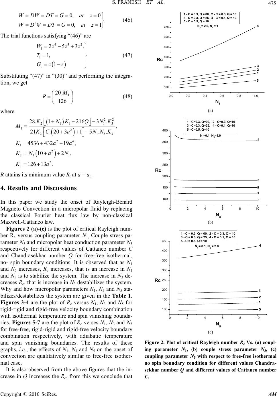

S. PRANESH ET AL.
475





1,0
0,0
2zatGDTWDW
zatGDTDWW (46)
The trial functions satisfying “(46)” are

432
1
1
1
253,
1,
1
Wzzz
T
Gz z




 
(47)
Substituting “(47)” in “(30)” and performing the integra-
tion, we get






126
20 1
M
R (48)
where



22
21113
12
2153
24
1
2
23 1
2
3
28.12163 .,
21. 20315..
4536 43219,
102 ,
126 13.
K
NKQNK
M
K
Ca NNK
Kaa
KNa N
Ka





 


R attains its minimum value Rc at a = ac.
4. Results and Discussions
In this paper we study the onset of Rayleigh-Bénard
Magneto Convection in a micropolar fluid by replacing
the classical Fourier heat flux law by non-classical
Maxwell-Cattaneo law.
Figures 2 (a)-(c) is the plot of critical Rayleigh num-
ber Rc versus coupling parameter N1, Couple stress pa-
rameter N3 and micropolar heat conduction parameter N5
respectively for different values of Cattaneo number C
and Chandrasekhar number Q for free-free isothermal,
no- spin boundary conditions. It is observed that as N1
and N5 increases, Rc increases, that is an increase in N1
and N5 is to stabilize the system. The increase in N3 de-
creases Rc, that is increase in N3 destabilizes the system.
Why and how micropolar parameters N1, N3 and N5 sta-
bilizes/destabilizes the system are given in the Table 1.
Figures 3-4 are the plot of Rc versus N1, N3 and N5 for
rigid-rigid and rigid-free velocity boundary combination
with isothermal temperature and spin vanishing bounda-
ries. Figures 5-7 are the plot of Rc verses N1, N3 and N5
for free-free, rigid-rigid and rigid-free velocity boundary
combination respectively, with adiabatic temperature
and spin vanishing boundaries. The results of these
graphs, i.e. , the effects of N1, N3 and N5 on the onset of
convection are qualitatively similar to free-free isother-
mal case.
It is also observed from the above figures that the in-
crease in Q increases the Rc, from this we conclude that
0.0 0.20.4 0.6 0.8 1.0
100
200
300
400
500
600
700
N
3
= 2.0, N
5
= 1
1 - C = 0.3, Q = 00, 2 - C = 0.3, Q = 1 0
3 - C = 0.3, Q = 25, 4 - C = 0.1, Q = 1 0
5 - C = 0.5, Q = 10
5
4
3
2
1
Rc
N
1
(a)
0246810
100
150
200
250
300
350
400
N
1
=0.1, N
5
=1.0
1 - C=0.3, Q=00, 2 - C =0.3, Q =10
3 - C=0.3, Q=25, 4 - C =0.1, Q =10
5 - C=0.5, Q=10
5
4
2
3
1
Rc
N
3
(b)
0246810
100
150
200
250
300
350
400
450
N
1
= 0.1, N
3
= 2.0
5
4
3
2
1
1 - C = 0.3, Q = 00, 2 - C = 0.3, Q = 10
3 - C = 0.3, Q = 25, 4 - C = 0.1, Q = 10
5 - C = 0.5, Q = 10
Rc
N
5
(c)
Figure 2. Plot of critical Rayleigh number Rc Vs. (a) coupl-
ing parameter N1, (b) couple stress parameter N3, (c)
coupling parameter N5 with respect to free-free isothermal
no spin boundary condition for different values Chandra-
sekhar number Q and different values of Cattaneo number
C.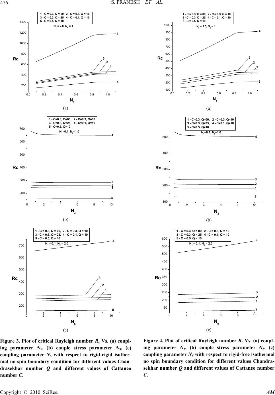

S. PRANESH ET AL.
476
0.0 0.2 0.4 0.6 0.8 1.0
200
400
600
800
1000
1200
1400
N
3
= 2.0, N
5
= 1
1 - C = 0.3, Q = 00, 2 - C = 0 .3, Q = 10
3 - C = 0.3, Q = 25, 4 - C = 0 .1, Q = 10
5 - C = 0.5, Q = 10
5
4
1
2
3
Rc
N
1
(a)
0246810
200
300
400
500
600
700
1 - C=0.3, Q=00, 2 - C=0.3, Q=10
3 - C=0.3, Q=25, 4 - C=0.1, Q=10
5 - C=0.5, Q=10
N
1
=0.1, N
5
=1.0
5
4
3
2
1
Rc
N
3
(b)
0246810
200
300
400
500
600
700 N
1
= 0.1, N
3
= 2.0
1 - C = 0.3, Q = 00, 2 - C = 0.3, Q = 1 0
3 - C = 0.3, Q = 25, 4 - C = 0.1, Q = 1 0
5 - C = 0.5, Q = 10
5
4
3
2
1
Rc
N
5
(c)
Figure 3. Plot of critical Rayleigh number Rc Vs. (a) coupl-
ing parameter N1, (b) couple stress parameter N3, (c)
coupling parameter N5 with respect to rigid-rigid isother-
mal no spin boundary condition for different values Chan-
drasekhar number Q and different values of Cattaneo
number C.
0.00.20.40.60.81.0
100
200
300
400
500
600
700
800
900
1000 N
3
= 2.0, N
5
= 1
1 - C = 0.3, Q = 00 , 2 - C = 0. 3, Q = 10
3 - C = 0.3, Q = 25 , 4 - C = 0. 1, Q = 10
5 - C = 0.5, Q = 10
5
4
3
2
1
Rc
N
1
(a)
0246810
100
200
300
400
500
N
1
=0.1, N
5
=1.0
1 - C=0.3, Q=00, 2 - C=0.3, Q=10
3 - C=0.3, Q=25, 4 - C=0.1, Q=10
5 - C=0.5, Q=10
5
4
3
2
1
Rc
N
3
(b)
0246810
150
200
250
300
350
400
450
500
550
600
N
1
= 0.1, N
3
= 2.0
1 - C = 0.3, Q = 00, 2 - C = 0.3, Q = 10
3 - C = 0.3, Q = 25, 4 - C = 0.1, Q = 10
5 - C = 0.5, Q = 10
5
4
3
2
1
Rc
N
5
(c)
Figure 4. Plot of critical Rayleigh number Rc Vs. (a) coupl-
ing parameter N1, (b) couple stress parameter N3, (c)
coupling parameter N5 with respect to rigid-free isothermal
no spin boundary condition for different values Chandra-
sekhar number Q and different values of Cattaneo number
C.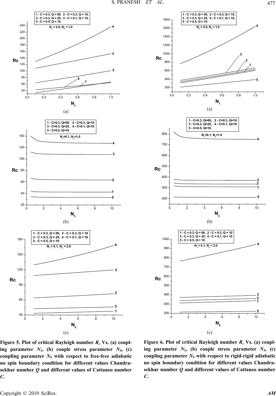

S. PRANESH ET AL.
477
0.0 0.2 0.4 0.6 0.8 1.0
40
60
80
100
120
140
160
180
200
220
240
5
4
3
2
1
N
3
= 2.0, N
5
= 1.0
1 - C = 0.3, Q = 00, 2 - C = 0.3, Q = 10,
3 - C = 0.3, Q = 25, 4 - C = 0.1, Q = 10,
5 - C = 0.5, Q = 10.
Rc
N
1
(a)
0246810
20
40
60
80
100
120
140
5
4
3
2
1
N
1
=0.1 , N
5
=1.0
1 - C=0.3, Q=00, 2 - C=0.3, Q=10
3 - C=0.3, Q=25, 4 - C=0.1, Q=10
5 - C=0.5, Q=10
N
3
Rc
(b)
0246810
30
60
90
120
150
180
1 - C = 0.3, Q = 00, 2 - C = 0.3, Q = 10
3 - C = 0.3, Q = 25, 4 - C = 0.1, Q = 10
5 - C = 0.5, Q = 10
N1 = 0.1, N3 = 2.0
5
4
3
2
1
Rc
N
5
(c)
Figure 5. Plot of critical Rayleigh number Rc Vs. (a) coupl-
ing parameter N1, (b) couple stress parameter N3, (c)
coupling parameter N5 with respect to free-free adiabatic
no spin boundary condition for different values Chandra-
sekhar number Q and different values of Cattaneo number
C.
0.0 0.20.4 0.60.8 1.0
200
400
600
800
1000
1200
1400
1600
1800
N3 = 2.0, N 5 = 1.0
1 - C = 0.3 , Q = 00 , 2 - C = 0 .3, Q = 10,
3 - C = 0.3 , Q = 25 , 4 - C = 0 .1, Q = 10,
5 - C = 0.5 , Q = 10 .
5
4
3
21
Rc
N
1
(a)
0246810
200
300
400
500
600
700
800 N
1
=0.1, N
5
=1.0
1 - C=0.3, Q=00, 2 - C =0.3, Q =10
3 - C=0.3, Q=25, 4 - C =0.1, Q =10
5 - C=0.5, Q=10
4
5
3
2
1
N3
Rc
(b)
0246810
200
300
400
500
600
700
800
900
1000
N
1
= 0.1, N
3
= 2.0
1 - C = 0.3, Q = 00, 2 - C = 0.3, Q = 10
3 - C = 0.3, Q = 25, 4 - C = 0.1, Q = 10
5 - C = 0.5, Q = 10
5
4
3
2
1
Rc
N
5
(c)
Figure 6. Plot of critical Rayleigh number Rc Vs. (a) coupl-
ing parameter N1, (b) couple stress parameter N3, (c)
coupling parameter N5 with respect to rigid-rigid adiabatic
no spin boundary condition for different values Chandra-
sekhar number Q and different values of Cattaneo number
C.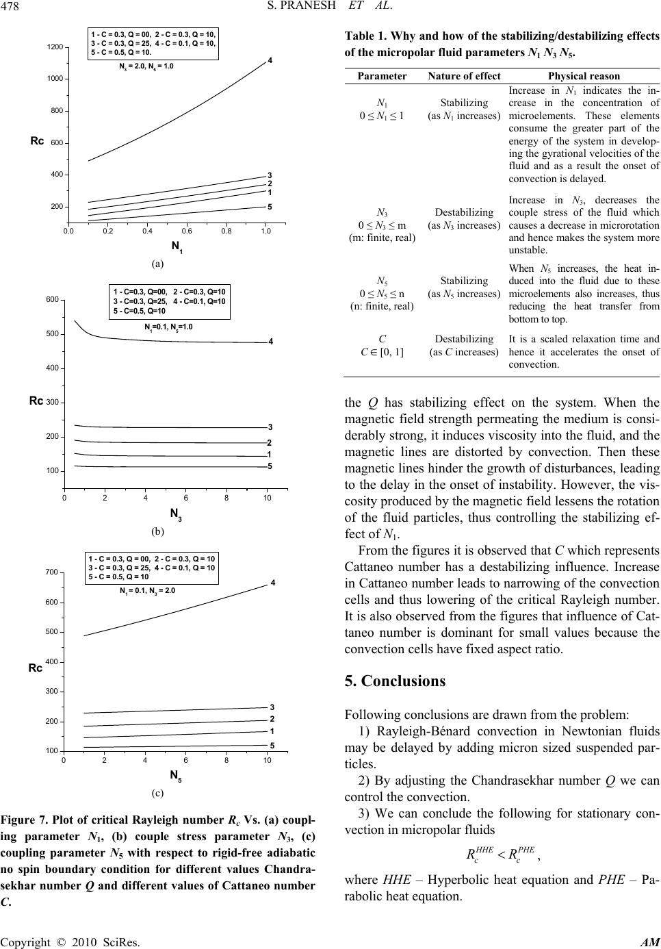

S. PRANESH ET AL.
478
0.0 0.2 0.4 0.6 0.8 1.0
200
400
600
800
1000
1200
5
4
3
2
1
N
3
= 2.0, N
5
= 1.0
1 - C = 0.3, Q = 00, 2 - C = 0.3, Q = 10,
3 - C = 0.3, Q = 25, 4 - C = 0.1, Q = 10,
5 - C = 0.5, Q = 10.
Rc
N
1
(a)
0246810
100
200
300
400
500
600
N
1
=0.1, N
5
=1.0
1 - C=0.3, Q=00, 2 - C=0.3, Q=10
3 - C=0.3, Q=25, 4 - C=0.1, Q=10
5 - C=0.5, Q=10
5
4
3
2
1
Rc
N
3
(b)
0246810
100
200
300
400
500
600
700
N
1
= 0.1, N
3
= 2.0
1 - C = 0.3, Q = 00, 2 - C = 0.3, Q = 10
3 - C = 0.3, Q = 25, 4 - C = 0.1, Q = 10
5 - C = 0.5, Q = 10
5
4
3
2
1
Rc
N
5
(c)
Figure 7. Plot of critical Rayleigh number Rc Vs. (a) coupl-
ing parameter N1, (b) couple stress parameter N3, (c)
coupling parameter N5 with respect to rigid-free adiabatic
no spin boundary condition for different values Chandra-
sekhar number Q and different values of Cattaneo number
C.
Table 1. Why and how of the stabilizing/destabilizing effects
of the micropolar fluid parameters N1 N3 N 5.
Parameter Nature of effect Physical reason
N1
0 ≤ N1 ≤ 1
Stabilizing
(as N1 increases)
Increase in N1 indicates the in-
crease in the concentration o
f
microelements. These elements
consume the greater part of the
energy of the system in develop-
ing the gyrational velocities of the
fluid and as a result the onset o
f
convection is delayed.
N3
0 ≤ N3 ≤ m
(m: finite, real)
Destabilizing
(as N3 increases)
Increase in N3, decreases the
couple stress of the fluid which
causes a decrease in microrotation
and hence makes the system more
unstable.
N5
0 ≤ N5 ≤ n
(n: finite, real)
Stabilizing
(as N5 increases)
When N5 increases, the heat in-
duced into the fluid due to these
microelements also increases, thus
reducing the heat transfer fro
m
bottom to top.
C
C

[0, 1]
Destabilizing
(as C increases)
It is a scaled relaxation time and
hence it accelerates the onset o
f
convection.
the Q has stabilizing effect on the system. When the
magnetic field strength permeating the medium is consi-
derably strong, it induces viscosity into the fluid, and the
magnetic lines are distorted by convection. Then these
magnetic lines hinder the growth of disturbances, leading
to the delay in the onset of instability. However, the vis-
cosity produced by the magnetic field lessens the rotation
of the fluid particles, thus controlling the stabilizing ef-
fect of N1.
From the figures it is observed that C which represents
Cattaneo number has a destabilizing influence. Increase
in Cattaneo number leads to narrowing of the convection
cells and thus lowering of the critical Rayleigh number.
It is also observed from the figures that influence of Cat-
taneo number is dominant for small values because the
convection cells have fixed aspect ratio.
5. Conclusions
Following conclusions are drawn from the problem:
1) Rayleigh-Bénard convection in Newtonian fluids
may be delayed by adding micron sized suspended par-
ticles.
2) By adjusting the Chandrasekhar number Q we can
control the convection.
3) We can conclude the following for stationary con-
vection in micropolar fluids
PHE
c
HHE
cRR,
where HHE – Hyperbolic heat equation and PHE – Pa-
rabolic heat equation.

S. PRANESH ET AL.
479
4) We also find that
FF
c
RF
c
RR
cRRR 
where the superscripts correspond to the three different
velocity boundary combinations. The above qualitative
results are true for both isothermal and adiabatic boun-
daries.
5) The non-classical Maxwell-Cattaneo heat flux law
involves a hyperbolic type heat transport equation that
predicts finite speeds of heat wave propagation (see [29]).
Hence it does not suffer from the physically unaccepta-
ble draw back of infinite heat propagation speed pre-
dicted by the parabolic heat equation. The classical
Fourier flux law overpredicts the critical Rayleigh num-
ber compared to that predicted by the non-classical law.
6. Acknowledgement
The authors like to thank management of Christ Univer-
sity for their support in completing this work. Second
author Kiran would like to thank Principal, Christ Junior
College for deputing him for Ph.D.
7. References
[1] J. C. Maxwell, “On the Dynamical Theory of Gases,” The
Philosophical Transactions of the Royal Society, Vol. 157,
1867, pp. 49-88.
[2] C. Cattaneo, “Sulla Condizione Del Calore,” Atti Del
Semin. Matem. E Fis. Della Univ. Modena, Vol. 3, 1948,
pp. 83-101.
[3] K. A. Lindsay and B. Straughan, “Acceleration Waves
and Second Sound in a Perfect Fluid,” Archive for Ra-
tional Mechanics and Analysis, Vol.68, 1978, pp 53-87.
[4] B. Straughan and F. Franchi, “Bénard Convection and the
Cattaneo Law of Heat Conduction,” Proceedings of the
Royal Society of Edinburgh, Vol. 96A, 1984, pp. 175-
178.
[5] G. Lebon and A. Cloot, “A Nonlinear Stability Analysis
of the Bénard-Marangoni Problem,” Journal of Fluid
Mechanics, Vol. 145, 1984, pp. 447-469.
[6] P. G. Siddheshwar, “Rayleigh Benard Convection in a
Second Order Ferromagnetic Fluid with Second Sound,”
Proceedings of 8th Asian Congress of Fluid Mechanics,
Shenzen, December 6-10, 1999, p. 631.
[7] S. Pranesh, “Effect of Second Sound on the Onset of
Rayleigh-Bénard Convection in a Coleman-Noll Fluid,”
Mapana Journal of Science, Vol. 7, No. 2, 2008, pp. 1-9.
[8] P. C. Dauby, M. Nelis and G. Lebon, “Generalized
Fourier Equations and Thermoconvective Instabilities,”
Revista Mexicana de Fisica, Vol. 48, 2001, pp. 57-62.
[9] B. Straughan, “Oscillatory Convection and the Cattaneo
Law of Heat Conduction,” Ricerche di Matematica, Vol.
58, No. 2, 2009, pp. 157-162.
[10] P. Puri and P. M. Jordan, “Stokes’ First Problem for a
Dipolar Fluid with Nonclassical Heat Conduction,” Jour-
nal of Engineering Mathematics, Vol. 36, No. 3, 1999, pp.
219-240.
[11] P. Puri and P. M. Jordan, “Wave Structure in Stokes
Second Problem for Dipolar Fluid with Nonclassical Heat
Conduction,” Acta Mechanica, Vol. 133, No. 1-4, 1999,
pp. 145-160.
[12] P. Puri and P. K. Kythe, “Nonclassical Thermal Effects in
Stokes Second Problem,” Acta Mechanica, Vol. 112, No.
1-4, 1995, pp. 1-9.
[13] P. Puri and P. K. Kythe, “Discontinuities in Velocity
Gradients and Temperature in the Stokes First Problem
with Nonclassical Heat Conduction,” Quarterly of Ap-
plied Mathematics, Vol. 55, No. 1, March 1997, pp. 167-
176.
[14] A. C. Eringen, “Simple Microfluids,” International Jour-
nal of Engineering Science, Vol. 2, No. 2, 1964, pp.
205-217.
[15] A. C. Eringen, “Theory of Thermomicrofluids,” Journal
of Mathematical Analysis and Applications, Vol. 38, No.
2, May 1972, pp. 480-496.
[16] A. C. Eringen, “Microcontinuum Field Theory,” Springer
Verlag, New York, 1999.
[17] H. Power, “Bio-Fluid Mechanics, Advances in Fluid
Mechanics,” W. I. T. Press, U. K., 1995.
[18] G. Lukaszewicz, “Micropolar Fluid Theory and Applica-
tions,” Birkhauser Boston, Boston, 1999.
[19] G. Ahmadi, “Stability of a Micropolar Fluid Layer
Heated from Below,” International Journal of Engineer-
ing Science, Vol. 14, No. 1, January 1976, pp. 81-89.
[20] Datta and V. U. K. Sastry, “Thermal Instability of a Ho-
rizontal Layer of Micropolar Fluid Heated from Below,”
International Journal of Engineering Science, Vol. 14,
No. 7, 1976, pp. 631-637.
[21] A. Perez Garcia and J. M. Rubi, “On the Possibility of
Overstable Motions of Micropolar Fluids Heated from
Below,” International Journal of Engineering Science,
Vol. 20, No. 7, 1982, pp. 873-878.
[22] L. E. Payne and B. Straughan, “Critical Rayleigh Num-
bers for Oscillatory and Nonlinear Convection in an In-
stropic Thermomicropolar Fluid,” International Journal
of Engineering Science, Vol. 27, 1989, p. 827.
[23] G. Lebon and C. Perez-Garcia, “Convective Instability of
a Micropolar Fluid Layer by the Method of Energy,” In-
ternational Journal of Engineering Science, Vol. 19, No.
10, 1981, pp. 1321-1329.
[24] S. Pranesh, “Effects of Suction-Injection-Combination
(SIC) on the Onset of Rayleigh-Bénard Magnetoconvec-
tion in a Fluid with Suspended Particles,” International
Journal of Engineering Science, Vol. 41, No. 15, Sep-
tember 2003, pp. 1741-1766.
[25] P. G. Siddheshwar and S. Pranesh, “Effects of a Non-
Uniform Basic Temperature Gradient on Rayleigh-
Bénard Convection in a Micropolar Fluid,” International
Journal of Engineering Science, Vol. 36, No. 11, Sep-
tember 1998, pp. 1183- 1196.
[26] P. G. Siddheshwar and S. Pranesh, “Suction-Injection

S. PRANESH ET AL.
480
Effects on the Onset of Rayleigh-Bénard-Marangoni
Convection in a Fluid with Suspended Particles,” Acta
Mechanica, Vol. 152, No. 1-4, 2001, pp. 241-252.
[27] P. G. Siddheshwar and S. Pranesh, “Magnetoconvection
in Fluids with Suspended Particles under 1g and G,” In-
ternational Journal of Aerospace Science and Technolo-
gy, Vol. 6, No. 2, February 2001, pp. 105-114.
[28] P. G. Siddheshwar and S. Pranesh, “Effect of Tempera-
ture/Gravity Modulation on the Onset of Magneto Con-
vection in Weak Electrically Conducting Fluids with In-
ternal Angular Momentum,” Journal of Magnetism and
Magnetic Materials, Vol. 192, No. 1, February 1999, pp.
159-176.
[29] Lawrence C. Evans, “Partial Differential Equations
(Schaum’s Outline Series),” Tata McGraw Hill, India,
2010.