Journal of Intelligent Learning Systems and Applications, 2010, 2, 200-211
doi:10.4236/jilsa.2010.24023 Published Online November 2010 (http://www.scirp.org/journal/jilsa)
Fast Variable Selection by Block Addition and
Block Deletion
Takashi Nagatani, Seiichi Ozawa*, Shigeo Abe*
Graduate School of Engineering, Kobe University, Rokkodai, Nada, Kobe, Japan
Received August 20th, 2010; revised September 25th, 2010; accepted September 27th, 2010.
ABSTRACT
We propose the threshold updating method for terminating variable selection and two variable selection methods. In the
threshold updating method, we update th e threshold value when the approximatio n error smaller than the current thre-
shold value is obtained. The first variable selection method is the combination of forward selection by block addition
and backward selection by block deletion. In this method, starting from the empty set of the input variables, we add
several input variables at a time until the approximation error is below the threshold value. Then we search deletable
variables by block deletion. The second method is the co mbination of the first method and variable selection by Linear
Programming Support Vector Regressors (LPSVRs). By training an LPSVR with linear kernels, we evaluate the weights
of the decision function and delete the input variables whose associated absolute weights are zero. Then we carry out
block addition and block deletion.
By computer experiments using benchmark data sets, we show that the proposed methods can perform faster variable
selection than the method only using block deletion, and that by the threshold updating method, the approximation er-
ror is lower than that by the fixed threshold method. We also compare our method with an imbedded method, which
determines the optimal variables during training, and show that our method gives comparable or better variable selec-
tion perf ormance.
Keywords: Backward Selection, Forward Selection, Least Squares Support Vector Machines, Linear Programming
Support Vector Machines, Support Vector Machines, Variable Selection
According to the selection criterion used, the variable
selection methods are classified into wrapper methods
and filter methods. Wrapper methods use the recognition
rate as the selection criterion and filter methods use the
selection criterion other than the recognition rate. Wrap-
per methods provide good generalization ability but usu-
ally at a much larger computational cost. Although the
computational cost of the filter methods may be small, it
will take a risk of selecting a subset of input variables
that may deteriorate the generalization ability of the re-
gressor.
1. Introduction
Function approximation estimates a continuous value for
the given inputs based on the relationship acquired from
a set of input-output pairs. As a tool to perform function
approximation, Support Vector Machines (SVMs) [1,2]
proposed by Vapnik attract much attention. Although
SVMs are developed for pattern recognition, they are
extended to solving function approximation problems
such as Support Vector Regressors (SVRs) [3], Least
Squares Support Vector Regressors (LSSVRs) [4], and
Linear Programming Support Vector Regressors
(LPSVRs) [5].
Wrapper and filter methods are used before training
regressors. But because SVRs are trained by solving op-
timization problems, imbedded methods, which select
variables during training are developed [6].
In developing a regressor, we may encounter problems
such as the high computational cost caused by a large
number of input variables and deterioration of the gener-
alization ability by redundant input variables. Variable
selection is one of the effective ways in reducing com-
putational complexity and improving the generalization
ability of the regressor.
Either by wrapper or filter methods, it is hard to test
the performance of all the subsets of input variables.
Thus, we generally perform backward selection or for-
ward selection. There is also a combination of forward
selection with backward selection [7,8]. In [7], sequential

Fast Variable Selection by Block Addition and Block Deletion201
forward selection is applied l times followed by r times
sequential backward selection, where l and r are fixed
integer values.
To speed up wrapper methods, some variable selection
methods using LPSVRs with linear kernels [9] are pro-
posed. For simplicity hereafter we call LPSVRs with
linear kernels linear LPSVRs. LPSVRs are usually used
to preselect input variables. After training linear LPSVRs,
input variables are ranked according to the absolute val-
ues of the weights and the input variables with small
absolute values are deleted. But because nonlinear func-
tion approximation problems are approximated by linear
LPSVRs, the nonlinear relations may be overlooked. To
overcome this problem, in [9], the data set is divided into
20 subsets and for each subset the weight vector is ob-
tained by training a linear LPSVR. Then the variables
with large absolute weights that often appear among 20
subsets are selected for nonlinear function approxima-
tion.
Backward variable selection by block deletion (BD)
[10] can select useful input variables faster than the con-
ventional backward variable selection. This method uses
as a selection criterion the generalization ability esti-
mated by cross-validation. To speed up variable selection,
it deletes multiple candidate variables. However, by this
method also it is difficult to perform variable selection
for a high-dimensional data set. Furthermore, this
method set the approximation error of the validation set
using all the input variables as the threshold value.
Therefore, if the initial input variables include irrelevant
variables for function approximation, the threshold value
may not be appropriate and high generalization ability
may not be obtained by variable selection.
To overcome the above problems, in this paper, we
propose a threshold updating method and two variable
selection methods based on block deletion and block
addition of variables. In the threshold updating method,
first we set the threshold value with the approximation
error evaluated using all the variables. Then during vari-
able selection process, if the approximation error better
than the current threshold value is obtained, we update
the threshold value by the approximation error. This
prevents deleting useful variables and thus leads to find-
ing the variable set that shows approximation perform-
ance better than the initial set of variables.
To realize efficient variable selection for a high-di-
mensional data set, we combine forward selection with
block addition and backward selection with block dele-
tion. We set the threshold value of selection evaluating
the approximation error using all the variables. Starting
from the empty set of variables, we estimate the ap-
proximation error when one input variable is temporarily
added to the selected set of variables and rank the vari-
ables in the ascending order of the approximation errors.
Then we add several high-ranked variables at a time and
rank the remaining variables. We iterate adding variables
and ranking remaining variables and terminate addition
when the approximation error is below the threshold
value.
After forward selection is finished, we delete variables,
by block deletion, that are redundantly added. Namely,
we rank variables with the ascending order of approxi-
mation errors deleting one input variable temporarily,
and delete high-ranked variables simultaneously.
To further speedup variable selection for a large num-
ber of input variables, we combine variable selection by
linear LPSVRs with block addition and block deletion.
Namely, we train a linear LPSVM using all the input
variables and delete the input variables whose associated
absolute weights are zero. After deletion, we compare
the approximation error for the selected variable set with
the threshold value. If the approximation error is above
the threshold value, we add variables by block addition
and then delete redundant variables by block deletion. If
the approximation error is below the threshold we delete
variables by block deletion.
In Section 2, we discuss the selection criteria and the
stopping conditions of the proposed method. Then in
Sections 3 and 4 we discuss the proposed methods, and
in Section 5, we show the results of computer experi-
ments using benchmark data sets. Finally in Section 6,
we conclude our work.
2. Selection Criteria and Stopping
Conditions
How and when to stop variable selection is one of the
important problems in variable selection. To obtain a set
of variables whose generalization ability is comparable
with or better than that of the initial set of variables, as
the selection criterion we use the approximation error of
the validation data set in cross-validation.
One way to obtain the smallest set of variables with
high generalization ability is by the fixed threshold value.
To do this, before variable selection, we set the threshold
value for the selection criterion evaluating the approxi-
mation error using all the variables. Let the threshold be
T. Then T is determined by
m
ET

, (1)
where m is the number of initial input variables and Em is
the approximation error of the validation set by
cross-validation. We fix T to Em throughout variable se-
lection and delete variables so long as the approximation
error of the current set of variables is below the threshold
or add variables so long as the approximation error is
above the threshold value. This method is called the fixed

Fast Variable Selection by Block Addition and Block Deletion
202
threshold method.
By the fixed threshold method, if the initial set of va-
riables includes irrelevant or redundant variables, the
threshold value calculated using all the variables might
give a conservative threshold value. Namely, if these
variables are deleted, we may obtain the approximation
error smaller than that with the initial set of variables. To
obtain a set of variables whose generalization ability is
smaller than that of the initial set of variables, we update
the threshold value when we obtain the approximation
error smaller than the threshold value as follows. Let the
current approximation error with j input variables be Ej.
Then if
TE j, (2)
we consider Ej as a new threshold value, that is, we set
j
ET  (3)
and continue variable selection. We call this method the
threshold updating method.
By the threshold updating method, the obtained set of
variables gives a smaller approximation error for the vali-
dation data set than that by the fixed threshold method.
But the number of selected variables may increase.
3. Variable Selection by Block Addition and
Block Deletion
If for a given approximation problem the number of input
variables is large, backward selection will be inefficient.
To speed up variable selection in such a situation, in the
following we discuss the first proposed method called
variable selection by block addition and block deletion
(BABD), which add and delete multiple variables ac-
cording to the variable ranking.
3.1. Idea
Suppose for a function approximation problem with m
variables, we select k variables. We examine the compu-
tational complexity of selecting the set of variables either
by sequential forward or backward selection with some
appropriate selection criterion. First we consider select-
ing k variables by sequential forward selection. Then
starting with the empty set, we temporally add one vari-
able at a time and evaluate the selection criterion, and
permanently add one variable with the best selection
criterion. In this method we need to evaluate selection
criterion m + (m 1) ++ (m k + 1) = k(2m k + 1)/2
times. In this case the number of variables used for
evaluating the criterion changes from 1 to k.
By sequential backward selection, starting from m
variables, we delete one variable temporarily at a time
and evaluate the selection criterion, and permanently
delete one variable with the best selection criterion. By
this method we need to delete (m k) variables. The
number of evaluations of the selection criterion is k(2m
k + 1)/2, which is the same as that by forward selection.
However, the number of variables used for evaluating the
selection criterion changes from m to m k. Therefore,
for k < m/2, forward selection will be faster than back-
ward selection. This tendency will be prominent for the
case where k m/2. 
From the standpoint of quality of the set of selected
variables, backward selection, which deletes irrelevant or
redundant variables from the variable set considering the
relation between the remaining variables, is more stable
than forward selection, which selects variables which are
important only for the selected variables, not considering
the relation with the unselected variables. For instance,
the variable that is selected first will be the best if only
one variable is used. But as variables are added, it may
be redundant. Therefore, to speed up backward selection,
we use forward selection as a pre-selector and afterwards,
for the set of selected variables we perform backward
selection. To speedup forward and backward selection
processes, we delete or add multiple variables at a time
and repeat addition or deletion until the stopping condi-
tion is satisfied.
3.2. Method
We explain BABD for the fixed threshold method. First,
we calculate the approximation error Em from the initial
set of input variables Im = {1,…, m} and set the threshold
value of the stopping condition T=Em. We start from the
empty set of selected variables. Assume that we have
selected j variables. Thus the set of input variables is I j.
Then we add the ith input variable in set I m – I j tempo-
rarily to I j and calculate E jiadd, where iadd indicates that
the ith input variable is added to the variable set. Then
we rank the variables in I m – I j in the ascending order of
the approximation errors. We call this ranking variable
ranking V j.
We add k (k

{1, 21,…,2A}) input variables from the
top of V j to the variable set temporarily, where 2A

m
and A is a user-defined parameter, which determines the
number of added candidates. We compare the error E j+k
with the value of threshold T. If
T
Ekj

, (4)
we add the variables to the variable set.
If (4) is not satisfied for k=1, 21,…, 2A, we check if for
some k the approximation error is decreased by adding k
variables to I j :
.
jkj EE   (5)
Here we assume that E 0 =

. If it is satisfied let

Fast Variable Selection by Block Addition and Block Deletion203
ij
iEk Al



2,,2,1
minarg

(6)
and we add to I j the first k variables in the variable rank-
ing. Then the current set of selected variables is I j+k. We
iterate the above procedure for I j+k until (4) is satisfied.
If (5) is not satisfied, we consider that block addition
of variables has failed and perform block deletion from
the initial set of variables. This is because if the addition
of variables that does not improve the approximation
accuracy continues, the efficiency of variable selection is
impaired. Thus, we finish variable addition in one fail-
ure.
Let the set of variables obtained after block addition
be I j. If block addition has failed, we set I j = I m. Now by
block deletion we delete redundant variables from I j. The
reason for block deletion is as follows. In block addition,
we evaluate variable ranking by temporarily adding one
input variable and we add multiple, high-ranked vari-
ables. Namely, in block addition we do not check corre-
lation of variables added at the same time. Thus, redun-
dant variables may be added by block addition.
We delete the ith variable in I j temporarily from I j and
calculate E jidel, where E jidel is the approximation error
when we delete the ith variable from I j. Then we con-
sider the input variables that satisfy
TE j
i
del (7)
as candidates of deletion and generate the set of input
variables that are candidates for deletion by
},|{ del
jj
i
jIiTEiS  (8)
We rank the candidates in the ascending order of E jidel
and delete all the candidates from I j temporarily. We
compare the error E j’ with the threshold T, where j' is the
number of input variables after the deletion. If
TE j
 (9)
block deletion has succeeded and we delete the candidate
variables permanently from I j. If block deletion has
failed, we backtrack and delete half of the variables pre-
viously deleted. We iterate the procedure until block
deletion succeeds. When the accuracy is not improved by
deleting any input variable, we finish variable selection.
In the threshold updating method, we update the
threshold value by (3) if for I j (2) is satisfied.
In the following, we show the algorithm of BABD.
The difference between the fixed threshold method and
the threshold updating method is shown in Steps 3 and 6.
Block Addition
Step 1 Calculate Em for Im. Set T = Em, j = 0, and E 0 =

.
And go to Step 2.
Step 2 Add the ith input variable in I m – I j temporarily to
I j, calculate E jiadd, and generate V j. Set k=1 and go
to Step 3.
Step 3 According to the fixed threshold or threshold up-
dating method, do the following.
For the fixed threshold method Add the k input
variables from the top of V j to I j, calculate E j+k
and compare it with the threshold T. If (4) is sat-
isfied, set j

j + k and go to Step 4. Otherwise, if
k < 2A, set k

2 k, and repeat Step 3. If k = 2A
and (5) is satisfied, add the k variables to I j, where
k is given by (6), and go to Step 2. If (5) is not
satisfied, set j

m and go to Step 4.
For the threshold updating method Calculate
E j+k (k = 1,21,…, 2A) and if (5) is satisfied for (6),
set j

j + k, T

E j and go to Step 2. Otherwise,
if T = E j go to Step 4. And if T < E j, set j

m
and go to Step 4.
Block Deletion
Step 4 Delete temporarily the ith input variable in I j and
calculate E jidel.
Step 5 Calculate S j. If S j is empty, stop variable selection.
If only one input variable is included in S j, set I j-1
= I j  S j, j

j 1 and go to Step 4. If S j has more
than one input variable, generate V j and go to
Step 6.
Step 6 Delete all the variables in V j from I j: I j’ = I j  V j,
where j' = j  |V j| and |V j| denotes the number of
elements in V j. Then, calculate E j’ and if (9) is not
satisfied, go to Step 7. Otherwise, do the follow-
ing.
For the fixed threshold method Update j with j'
and go to Step 4.
For the threshold updating method Update j
with j', T

E j’, and go to Step 4.
Step 7 Let V' j include the upper half elements of V j. Set
I j’ = I j  { V' j }, where V' j is the set that includes
all the variables in V' j and j' = j  |{ V' j }|. Then,
if (9) is satisfied, delete input variables in V' j and
go to Step 4 updating j with j'. Otherwise, update
V j with V' j and iterate Step 7 so long as (9) is sat-
isfied.
3.3. Complexity and Suitability of the Method
To make discussions simple, we consider the fixed thre-
shold method. First consider the complexity of block
addition in contrast to sequential addition. For m vari-
ables, assume that only one variable can satisfies the
stopping condition. By sequential addition we need to
evaluate the selection criterion m times and by selecting
one variable the algorithm stops. By block addition, the
selection criterion is evaluated m times and at the first

Fast Variable Selection by Block Addition and Block Deletion
204
The primal problem of the linear LPSVR is given by
minimize
 

M
iii
m
iiCwbQ
1
*
1
*)(||),,,(
 ξξw
block addition, one variable, which satisfies the stopping
condition, is added and block addition terminates. Thus,
the complexity of calculation is the same for the both
methods.
subject to ,,,1for Niby ii
T
i
 xw For the case where 2A (> 1) variables are successfully
added, by sequential addition, the selection criterion is
evaluated 2A (m  2A-1 + 1/2) times. Suppose that block
addition of 2A variables succeeds following A failures of
block addition. Then the selection criterion needs to be
calculated m + A times. Therefore, for A 1 block ad-
dition is faster. Here, we assume that the same sets of
variables are added for both methods. But because by
block addition the correlation between variables is not
considered, more than m + A times calculations may be
necessary. In this case added redundant variables will be
deleted by the subsequent block deletion.

,,,1for
*Niyb iii
T
 xw
where, xi and yi are the ith (i = 1, …, N) training input
and output, respectively, wi is the ith element of the
weight vector w associated with the ith input variable xi
of x, b is the bias term,  is the user-defined error thresh-
old, C is the margin parameter, and
 
i is the slack vari-
able associated with xi. As will be explained in Section
5.2, values of C and
 are determined by cross-valida-
tion.
In the decision function of the linear LPSVR, each in-
put variable xi is multiplied by an associated weight ele-
ment wi. Therefore, if the weight elements are zero, the
associated variables do not contribute to function ap-
proximation and we can delete these variables [11]. In
addition because the number of equality constrained
conditions is 2M, at most 2M weight elements take
non-zero values. Thus, if the number of input variables is
larger than 2M, by training the linear LPSVR, we can
delete at least m  2M variables whose weight elements
are zero. But if we use a linear SVR, the number of
non-zero variables is not restricted to 2M.
Consider backward selection. For m variables, assume
that we can only delete one variable, but 2i variables are
candidates of deletion. By sequential deletion, we need
to evaluate the selection criterion 2m  1 times but by
block deletion, 2m + i  1 times because of i times failures.
Thus, by block deletion we need to calculate the selec-
tion criterion i more times. This is the worst case. Now
consider the best case, where 2i variables are success-
fully deleted by block deletion and no further deletion is
possible. By block deletion, we need to calculate the
criterion m + 1 + m  2i = 2m  2i + 1 times, but by sequen-
tial deletion, m + (m  1) ++ (m  2i) + (m  2i  1) times.
Thus, for i > 1, block deletion is faster.
At first, we set the threshold of the stopping condition
T = Em from the initial set of variables Im. By training a
linear LPSVR, we calculate the weight elements wi (i= 1,
…, m) and delete the input variables with zero weights.
Therefore, the effect of block addition and block dele-
tion becomes prominent as many data are successfully
added or deleted.
We set jLP as the number of input variables after pre-
selection. Then we compare the current approximation
error EJLP with the threshold T. If
4. Variable Selection by Block Addition and Block
Deletion with LP SVRs TE LPj , (10)
If the number of input variables is very large, even block
addition or block deletion may be inefficient because
during variable selection the approximation error needs to
be estimated deleting or adding one input variable at a
time. To overcome this problem preselection of input
variables is often used [11]. We preselect variables by
LPSVRs with linear kernels before block addition and
deletion. We call this method variable selection by block
addition and block deletion with LPSVRs (BABD-LP). If
the input-output relations of the given problem are
nonlinear, we may not be able to obtain good initial set of
variables. This problem is solved by properly combining
preselection by the LPSVR with BABD. Namely, if the
approximation error obtained by preselection is not satis-
factory, we add variables by block addition to the set of
variables obtained by preselection. And if it is, we delete
variables by block deletion from the set.
we search more deletable variables by block deletion. If
(10) is not satisfied, we add the variables that improve
the approximation accuracy to the current variable set by
block addition. After block addition is finished we delete
variables by block deletion. In the threshold updating
method, if (10) is satisfied, we update T by EJLP.
In the following we show the algorithm of BABD-LP.
After preselection, block addition and block deletion are
performed. But since these procedures are the same as
those in Section 3.2, we do not repeat here.
Preselection
Step 1 Calculate Em for Im. Set T = Em and go to Step 2.
Step 2 Calculate wi (I = 1, …, m) by training the linear
LPSVR. From Im delete variables whose associ-
ated weight elements are zero. Let the resulting
set of variables obtained by preselection be I jLP .

Fast Variable Selection by Block Addition and Block Deletion
205
Step 3 Calculate E jLP for I jLP. If (10) is not satisfied, set
jjLP, E jE jLP, and go to Step 2 in Section 3.2.
Otherwise, do the following.
H(x, x') = g(x)T g(x) and  is a parameter for determining
the spread of the radius.
For LSSVRs, we need to optimize the values of the
margin parameter and the kernel parameter. But for
SVRs, in addition to the two parameter values, we need
to optimize the value of the
 tube parameter. Thus, us-
ing LSSVRs we can perform faster variable selection
than using SVRs.
For the fixed threshold method Set j

jLP and
go to Step 4 in Section 3.2.
For the threshold updating method Set j

jLP
and TE jLP and go to Step 4 in Section 3.2.
5. Performance Evaluation We determine the initial approximation error by five-
fold cross-validation changing the values of the kernel
and margin parameters. Namely, we train the LSSVR for
all pairs of parameter values and select the values that
realize the minimum approximation error for the valida-
tion data set.
In this section, we compare BABD and BABD-LP with
BD using benchmark data sets. We also compare the
proposed methods with the embedded method [9]. To
distinguish between the fixed threshold method and the
threshold updating method, we add subscript u to the
abbreviation of the proposed method, e.g., BABDu. Then to reduce computational cost of training the
LSSVR during variable selection, fixing the kernel pa-
rameter value, we optimize the margin parameter by
cross-validation. Thus, there is a possibility of improving
variable selection by determining both kernel and margin
parameter values, but with a considerable computation
cost.
5.1. Use of Least Squares Support Vector
Regressors as Regressors
By setting some appropriate selection criterion, BABD
can be used as a filter method but to obtain reliable set of
variables, in performance evaluation we use the ap-
proximation error for the validation data set evaluated by
cross-validation by Least Squares Support Vector Re-
gressors (LSSVRs). According to [10], the use of
LSSVRs or SVRs in variable selection or in evaluating
the approximation errors does not give much difference.
Therefore, in variable selection we use LSSVRs because
their training is faster than that of SVRs for small and
medium size regression problems.
5.2. Benchmark Data Sets and Evaluation
Conditions
We use the benchmark data sets shown in Table 1,
which lists the numbers of input variables, training data,
test data, and the type of data set. We also list the mini-
mum number of selected features found in the literature.
The bottom three data sets deal with pattern classifica-
tion and are used for comparing our methods with the
NLPSVM (Newton method for Linear Programming
SVM) [9].
The primal problem of LSSVR is given by
minimize 


N
ii
TC
1
2
22
1
 ww (11)
To examine that our proposed methods can delete re-
dundant variables, we modify the Mackey-Glass data set
[12], which is generated by a differential equation with-
out noise. We add 18 artificial redundant input variables
generated by a uniform random variable in [0,1] to the set.
Boston 5 and Boston 14 data sets [13] use the 5th and
14th input variables of the Boston data set as outputs,
respectively. Excluding the Mackey-Glass data set, these
subject to (12)
,,,1for)( Niby ii
T
i
 xgw
where g(x) is the mapping function that maps x into the
feature space. In training the LSSVR, we solve the set of
linear equations that is derived by transforming the pri-
mal problem into the dual problem. As a kernel function,
we use RBF kernels: H(x, x') = exp( -
 || x  x' ||2), where
Table 1. Specifications of data sets and selected features.
Data Set Inputs Train. Test Type Selected
Mackey-Grass [12] 22 500 500 regres. －
Boston5 [13,14] 13 506 － regres. －
Boston14 [13,14] 13 506 － regres. 4 [15]
Water Purification [12] 10 241 237 regres. －
Pyrimidines [16] 27 74 － regres. 5 [17]
Triazines [16] 60 186 － regres. 2 [17]
Phenetylamines [18] 628 22 － regres. 30 [19]
Orange Juice [20] 700 150 68 regres. 7 [21]
Ionosphere [16] 34 351 － class. 11.2 [9]
BUPA Liver [16] 6 345 － class. 4.9 [9]
Pima Indians [16] 8 768 － class. 4.9 [9]

Fast Variable Selection by Block Addition and Block Deletion 206
data sets are real data sets. In our experiments, except for
the Mackey-Glass, ionosphere, BUPA liver, and Pima
Indians data sets we combine the training data set with
the test data set and randomly divide the set into two. In
doing so, we make 20 pairs of training and test data sets
for the original one pair of training and test data sets.
We determine the values of the kernel parameter
 , the
error-threshold parameter
 , and the margin parameter C
by fivefold cross-validation.
In the experiment of the regression data sets, we
change
 = {0.1, 0.5, 1.0, 5.0, 10, 15, 20, 50, 100}, C =
{1, 10, 100, 1000, 5000, 104, 105} for LSSVRs. In the
experiment of the classification data sets, we change C =
{100, 1000, 5000, 104, 105, 106, 107, 108}.
Since we do not want to waste time in preselection and
since variable selection is improved by block addition
and block deletion, we set the parameters ranges for
LPSVRs as follows: C = {10, 10000} and
 = {0.01, 0.2}.
We set the user-parameter A according to the dimen-
sion of the data sets; A = 3 for the data sets with less than
100 input variables and A = 5 otherwise. The approxima-
tion error is measured by the mean absolute error.
We use an Athlon 64 XII 4800 + personal computer
(2GB memory, Linux operating system) in measuring
variable selection time.
5.3. Effect of Parameters
In applying BABD or BABDu we need to determine the
value of A. In this section, we investigate the effect of A
on the number of added variables and the approximation
error using the phenetylamines data set. Because the
number of input variables is 628, the maximum value of
A is 10. Table 2 shows the approximation error of the
validation data set after variable selection, the selected
variables and the numbers of variables selected by block
addition and block deletion. Since the results by BABDu
for A = 7 to 10 are the same as that by A = 6 and those by
BABD are the same as that by A = 2 to 10, we only list
the results for A = 1 to 6.
By BABD, two variables are selected by block addi-
tion and no variables are deleted by block deletion. But
by BABDu, the numbers of selected variables vary as the
value of A changes except for A = 2 and 3. For the value
of A larger than 3, some of the variables added by block
addition are deleted by block deletion. Variable selection
time is around five seconds by BABD and 30 to 60 sec-
onds by BABDu. By the fixed threshold method, the
change of A does not make much difference but by the
threshold updating method the results change according
to the change of A. Thus to obtain the best results we
need to determine the optimum value of A by
cross-validation. But because it will require much com-
putation time, in our following study we fix A = 5 with
variables larger than 100 and A = 3 otherwise, as stated
before.
5.4. Results for the Mackey-Glass Data Set
Table 3 shows the results for the Mackey-Glass 22 data
set. In the table, the columns “Before” and “After” list
the approximation errors before and after variable selec-
tion; the column “Vali.” lists the approximation errors
evaluated by cross-validation; “Test” lists the approxima-
tion errors for the test data sets; The column “Selected”
lists the input variables selected by variable selection;
The results in the column “Before” are the same for the
six variable selection methods, so we list the results only
in the first row among the six rows. The columns “LP,”
“BA,” and “BD” denote the numbers of variables after
Table 2. Effect of the value of A to the performance for the phenetylamines data set. The initial approximation error for
the validation data set is 0.156.
BABD BABDu
A Vali. Selected BA BD Vali. Selected BA BD
1 0.120 384, 404 2 2 0.057 124, 404, 604, … 13 13
2 0.156 123, 404 2 2 0.048 124, 330, 341, 404, … 11 11
3 0.156 123, 404 2 2 0.048 124, 330, 341, 404, … 11 11
4 0.156 123, 404 2 2 0.033 8, 60, 155, 328, 358, 364, 404, … 25 16
5 0.156 123, 404 2 2 0.025 8, 60, 157, 328, 330, 358, 404, … 45 22
6 0.156 123, 404 2 2 0.039 8, 155, 157, 341, 364, 604, … 74 28
Table 3. Performance for the Mackey-Glass data set.
Before After
Method Vali. Test Vali. Test Selected LP BA BD Time [s]
BD 0.042 0.038 0.029 0.029 2, 4
－ － 2 94
BABD 0.036 0.035 1, 2
－ 2 2 87
BABD-LP 0.029 0.029 2, 4 21 21 2 201
BDu 0.019 0.018 1, 2, 3, 4 － － 4 87
BABDu 0.018 0.018 1, 2, 3, 4 － 4 4 139
BABD-LPu 0.021 0.021 1, 2, 4 21 21 3 248

Fast Variable Selection by Block Addition and Block Deletion 207
selection by the LPSVR, block addition, and block dele-
tion, respectively. Thus, for the row “BABD-LP,” 21 in
the column “LP” means that by the LPSVR, 21 variables
are selected from 22 variables and 21 in the column
“BA,” means that because selection by the LPSVR does
not worsen the generalization ability evaluated by
cross-validation, variables are not added by block addi-
tion.
The first four variables are original input variables.
Thus, from the table no irrelevant variables are selected
by the proposed methods and preselection by the LPSVR
and block addition does not fail selecting variables. By
the fixed threshold method, the two variables are selected
to realize the approximation error of the validation data
set obtained by the initial 22 variables.
By the threshold updating method, the three or four
original variables are selected and the approximation er-
rors are decreased further. Thus the threshold updating
method is useful when redundant input variables are in-
cluded. Since the number of variables is 22, BD or BDu is
preferable from the standpoint of computation time.
5.5. Results for Function Approximation
Problems
We evaluate the regression problems listed in Table 1
from the average approximation errors, the average
number of selected variables, and the average training
time using the multiple data sets. Table 4 shows the re-
sult. The column “Num.” lists the number of input vari-
ables selected by variable selection; The column “Time”
lists the computation time.
We analyze the statistical difference of the approxima-
tion errors and the computation time by the Welch t-test
with a 5% significance level. We test the statistical dif-
ferences of the approximation errors between the initial
set of variables and the selected set of variables for the
validation data sets and the test data sets. If there is sig-
nificant difference, we mark the asterisk to the better re-
sult. If there are significant difference among the results
by BD, BABD, and BABD-LP or by BDu, BABDu, and
BABD-LPu, we change the font of the best result to bold.
For example, for the results of triazines data set the aster-
isks in the “After” “Vali.” column mean that the ap-
proximation errors of the validation sets after variable
selection are significantly smaller than those before vari-
able selection. And the asterisks for the BABD,
BABD-LP, and BABD-LPu results in the “Before” “Test”
column mean that the approximation errors before vari-
able selection are significantly smaller than those after
variable selection. Furthermore, the bold font in the
BABD-LP (BABD-LPu) row means that the computation
time of BABD-LP (BABD-LPu) is significantly shorter
than the other two methods.
From the table the computational time and the ap-
proximation errors of BD, BDu, BABD, and BABDu are
almost the same for the Boston 14, Boston 5, and water
purification data sets. This means that for low dimen-
sional data sets, there is not much difference between
forward selection and backward selection. But for
BABD-LP and BABD-LPu, it takes much time to train
LPSVRs and we cannot delete many variables by the
preselection. Therefore, BABD-LP and BABD-LPu are
ineffective for these data sets.
For the pyrimidines, triazines, and phenetylamines
problems one or two input variables are enough to get a
comparable accuracy as the initial threshold. In addition,
many input variables are deleted by preselection using
LPSVRs. Accordingly, BABD, BABDu, BABD-LP,
BABD-LPu can perform high-speed variable selection.
For the Orange juice problem, the standard deviations
BD
BABD
BABD-LP
Time (s)
500 10000
Approximation Error
BD
BABD
BABD-LP
Time (s)
500 10000
0
100
200
300
400
500
600
700
Number of Variables
3
3.5
4
4.5
5
5.5
Figure 1. Performance comparison for the orange juice data set by the fixed threshold method: (a) The approximation error;
(b) The number of selected variables.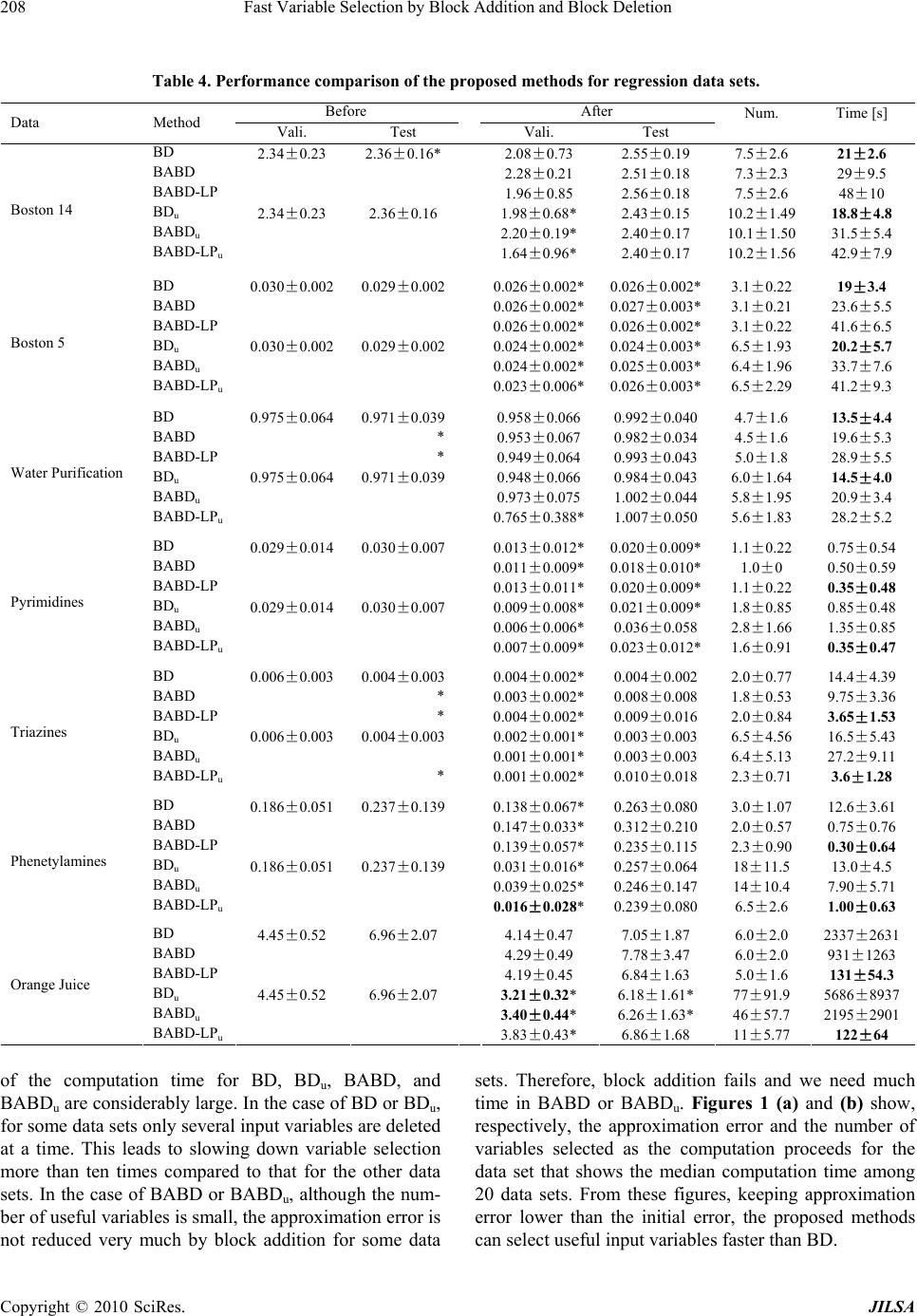

Fast Variable Selection by Block Addition and Block Deletion
208
Table 4. Performance comparison of the proposed methods for regression data sets.
Before After
Num. Time [s]
Data Method
Vali. Test Vali. Test
BD 2.34±0.23 2.36±0.16* 2.08±0.73 2.55±0.19 7.5±2.6 21±2.6
BABD 2.28±0.21 2.51±0.18 7.3±2.3 29±9.5
BABD-LP 1.96±0.85 2.56±0.18 7.5±2.6 48±10
BDu 2.34±0.23 2.36±0.16 1.98±0.68* 2.43±0.15 10.2±1.49 18.8±4.8
BABDu 2.20±0.19* 2.40±0.17 10.1±1.50 31.5±5.4
Boston 14
BABD-LPu 1.64±0.96* 2.40±0.17 10.2±1.56 42.9±7.9
BD 0.030±0.002 0.029±0.0020.026±0.002* 0.026±0.002* 3.1±0.22 19±3.4
BABD
0.026±0.002* 0.027±0.003* 3.1±0.21 23.6±5.5
BABD-LP 0.026±0.002* 0.026±0.002* 3.1±0.22 41.6±6.5
BDu 0.030±0.002 0.029±0.0020.024±0.002* 0.024±0.003* 6.5±1.93 20.2±5.7
BABDu
0.024±0.002* 0.025±0.003* 6.4±1.96 33.7±7.6
Boston 5
BABD-LPu 0.023±0.006* 0.026±0.003* 6.5±2.29 41.2±9.3
BD 0.975±0.064 0.971±0.039 0.958±0.066 0.992±0.040 4.7±1.6 13.5±4.4
BABD *0.953±0.067 0.982±0.034 4.5±1.6 19.6±5.3
BABD-LP *0.949±0.064 0.993±0.043 5.0±1.8 28.9±5.5
BDu 0.975±0.064 0.971±0.039 0.948±0.066 0.984±0.043 6.0±1.64 14.5±4.0
BABDu 0.973±0.075 1.002±0.044 5.8±1.95 20.9±3.4
Water Purification
BABD-LPu 0.765±0.388*1.007±0.050 5.6±1.83 28.2±5.2
BD 0.029±0.014 0.030±0.0070.013±0.012* 0.020±0.009* 1.1±0.22 0.75±0.54
BABD
0.011±0.009* 0.018±0.010* 1.0±0 0.50±0.59
BABD-LP 0.013±0.011* 0.020±0.009* 1.1±0.22 0.35±0.48
BDu 0.029±0.014 0.030±0.0070.009±0.008* 0.021±0.009* 1.8±0.85 0.85±0.48
BABDu 0.006±0.006*0.036±0.058 2.8±1.66 1.35±0.85
Pyrimidines
BABD-LPu 0.007±0.009* 0.023±0.012* 1.6±0.91 0.35±0.47
BD 0.006±0.003 0.004±0.0030.004±0.002*0.004±0.002 2.0±0.77 14.4±4.39
BABD *0.003±0.002*0.008±0.008 1.8±0.53 9.75±3.36
BABD-LP *0.004±0.002*0.009±0.016 2.0±0.84 3.65±1.53
BDu 0.006±0.003 0.004±0.0030.002±0.001*0.003±0.003 6.5±4.56 16.5±5.43
BABDu
0.001±0.001*0.003±0.003 6.4±5.13 27.2±9.11
Triazines
BABD-LPu *0.001±0.002* 0.010±0.018 2.3±0.71 3.6±1.28
BD 0.186±0.051 0.237±0.1390.138±0.067*0.263±0.080 3.0±1.07 12.6±3.61
BABD
0.147±0.033*0.312±0.210 2.0±0.57 0.75±0.76
BABD-LP 0.139±0.057*0.235±0.115 2.3±0.90 0.30±0.64
BDu 0.186±0.051 0.237±0.1390.031±0.016*0.257±0.064 18±11.5 13.0±4.5
BABDu
0.039±0.025*0.246±0.147 14±10.4 7.90±5.71
Phenetylamines
BABD-LPu 0.016±0.028*0.239±0.080 6.5±2.6 1.00±0.63
BD 4.45±0.52 6.96±2.07 4.14±0.47 7.05±1.87 6.0±2.0 2337±2631
BABD 4.29±0.49 7.78±3.47 6.0±2.0 931±1263
BABD-LP 4.19±0.45 6.84±1.63 5.0±1.6 131±54.3
BDu 4.45±0.52 6.96±2.07 3.21±0.32* 6.18±1.61* 77±91.9 5686±8937
BABDu 3.40±0.44* 6.26±1.63* 46±57.7 2195±2901
Orange Juice
BABD-LPu 3.83±0.43* 6.86±1.68 11±5.77 122±64
of the computation time for BD, BDu, BABD, and
BABDu are considerably large. In the case of BD or BDu,
for some data sets only several input variables are deleted
at a time. This leads to slowing down variable selection
more than ten times compared to that for the other data
sets. In the case of BABD or BABDu, although the num-
ber of useful variables is small, the approximation error is
not reduced very much by block addition for some data
sets. Therefore, block addition fails and we need much
time in BABD or BABDu. Figures 1 (a) and (b) show,
respectively, the approximation error and the number of
variables selected as the computation proceeds for the
data set that shows the median computation time among
20 data sets. From these figures, keeping approximation
error lower than the initial error, the proposed methods
can select useful input variables faster than BD.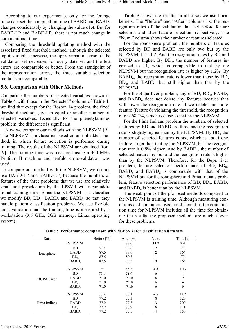

Fast Variable Selection by Block Addition and Block Deletion209
Table 5 shows the results. In all cases we use linear
kernels. The “Before” and “After” columns list the rec-
ognition rates of the validation data set before feature
selection and after feature selection, respectively. The
“Num.” column shows the number of features selected.
According to our experiments, only for the Orange
juice data set the computation time of BABD and BABDu
changes considerably by changing the value of A. But for
BABD-LP and BABD-LPu there is not much change in
computational time.
For the ionosphere problem, the numbers of features
selected by BD and BABD are only two but by the
NLPSVM it is 11.2. And the recognition rates by BD and
BABD are higher. By BDu, the number of features in-
creased to 11, which is comparable to that by the
NLPSVM but the recognition rate is higher by 1.2%. By
BABDu, the recognition rate is lower than those by BD,
BDu, and BABD, but still higher than that by the
NLPSVM.
Comparing the threshold updating method with the
associated fixed threshold method, although the selected
input variables increase, the approximation error of the
validation set decreases for every data set and the test
errors are comparable or better. From the standpoint of
the approximation errors, the three variable selection
methods are comparable.
5.6. Comparison with Other Methods
For the Bupa liver problem, any of BD, BDu, BABD,
and BABDu does not delete any features because that
will lower the recognition rate. If we delete one more
feature (feature 6) violating the threshold, the recognition
rate is 68.7%, which is close to that by the NLPSVM.
Comparing the numbers of selected variables shown in
Table 4 with those in the “Selected” column of Table 1,
we find that except for the Boston 14 problem, the fixed
threshold methods give an equal or smaller number of
selected variables. Especially for the phenetylamines
problem, the difference is significant. For the Pima Indians problem the numbers of selected
features by BD and BABD are three and the recognition
rate is slightly higher than by the NLPSVM. By BDu the
number of selected features is six, which is about one
feature larger than that by the NLPSVM, but the recogni-
tion rate is 0.8% higher. And by BABDu, the number of
selected features is four and the recognition rate is higher
than by the NLPSVM. Therefore, for the Bupa liver
problem, feature selection performance of BD, BDu,
BABD, and BABDu is comparable with that of the
NLPSVM but for the ionosphere and Pima Indians prob-
lem, feature selection performance of BD, BDu, BABD,
and BABDu is better than by the NLPSVM.
Now we compare our methods with the NLPSVM [9].
The NLPSVM is a classifier based on an imbedded me-
thod, in which feature selection is performed during
training. The results of the NLPSVM are obtained from
[9]. The training time was measured using a 400 MHz
Pentium II machine and tenfold cross-validation was
used.
To compare our method with the NLPSVM, we do not
use BABD-LP and BABD-LPu because the numbers of
features of the three problems that we use are relatively
small and preselection by the LPSVR will incur addi-
tional training time. Since the NLPSVM is a classifier
we modify BD, BDu, BABD, and BABDu so that they
handle pattern classification problems. We use fivefold
cross-validation and the training time is measured by a
workstation (3.6 GHz, 2GB memory, Linux operating
system).
The weak point of the proposed methods compared to
the NLPSVM is training time. Although measuring con-
ditions and computers used are different, if the computa-
tion time for NLPSVM includes all the time for obtain-
ing the results, the proposed methods are much slower
for these problems.
Table 5. Performance comparison with NLPSVM for classification data sets.
Data Before [%] After [%] Num. Time [s]
NLPSVM － 88.0 11.2 2.4
BD 87.5 88.6 2 72
BABD 87.5 88.6 2 164
BDu 87.5 89.2 11 79
Ionosphere
BABDu 87.5 88.3 9 165
NLPSVM － 68.8 4.8 1.13
BD 71.0 71.0 6 4
BABD 71.0 71.0 6 9
BDu 71.0 71.0 6 4
BUPA Liver
BABDu 71.0 71.0 6 9
NLPSVM 77.2 77.1 4.9 1.07
BD 77.2 77.3 3 120
BABD 77.2 77.3 3 200
BDu 77.2
77.9 6 111
Pima Indians
BABDu 77.2 77.5 4 150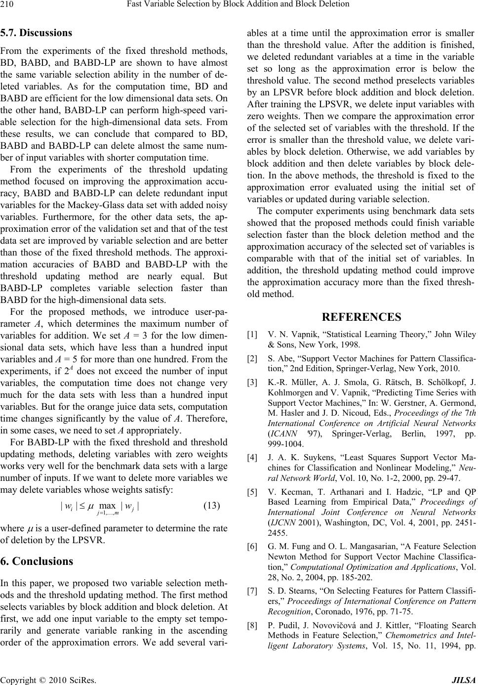

Fast Variable Selection by Block Addition and Block Deletion 210
5.7. Discussions
From the experiments of the fixed threshold methods,
BD, BABD, and BABD-LP are shown to have almost
the same variable selection ability in the number of de-
leted variables. As for the computation time, BD and
BABD are efficient for the low dimensional data sets. On
the other hand, BABD-LP can perform high-speed vari-
able selection for the high-dimensional data sets. From
these results, we can conclude that compared to BD,
BABD and BABD-LP can delete almost the same num-
ber of input variables with shorter computation time.
From the experiments of the threshold updating
method focused on improving the approximation accu-
racy, BABD and BABD-LP can delete redundant input
variables for the Mackey-Glass data set with added noisy
variables. Furthermore, for the other data sets, the ap-
proximation error of the validation set and that of the test
data set are improved by variable selection and are better
than those of the fixed threshold methods. The approxi-
mation accuracies of BABD and BABD-LP with the
threshold updating method are nearly equal. But
BABD-LP completes variable selection faster than
BABD for the high-dimensional data sets.
For the proposed methods, we introduce user-pa-
rameter A, which determines the maximum number of
variables for addition. We set A = 3 for the low dimen-
sional data sets, which have less than a hundred input
variables and A = 5 for more than one hundred. From the
experiments, if 2A does not exceed the number of input
variables, the computation time does not change very
much for the data sets with less than a hundred input
variables. But for the orange juice data sets, computation
time changes significantly by the value of A. Therefore,
in some cases, we need to set A appropriately.
For BABD-LP with the fixed threshold and threshold
updating methods, deleting variables with zero weights
works very well for the benchmark data sets with a large
number of inputs. If we want to delete more variables we
may delete variables whose weights satisfy:
1, ,
||max| |
i
jm
wj w



(13)
where  is a user-defined parameter to determine the rate
of deletion by the LPSVR.
6. Conclusions
In this paper, we proposed two variable selection meth-
ods and the threshold updating method. The first method
selects variables by block addition and block deletion. At
first, we add one input variable to the empty set tempo-
rarily and generate variable ranking in the ascending
order of the approximation errors. We add several vari-
ables at a time until the approximation error is smaller
than the threshold value. After the addition is finished,
we deleted redundant variables at a time in the variable
set so long as the approximation error is below the
threshold value. The second method preselects variables
by an LPSVR before block addition and block deletion.
After training the LPSVR, we delete input variables with
zero weights. Then we compare the approximation error
of the selected set of variables with the threshold. If the
error is smaller than the threshold value, we delete vari-
ables by block deletion. Otherwise, we add variables by
block addition and then delete variables by block dele-
tion. In the above methods, the threshold is fixed to the
approximation error evaluated using the initial set of
variables or updated during variable selection.
The computer experiments using benchmark data sets
showed that the proposed methods could finish variable
selection faster than the block deletion method and the
approximation accuracy of the selected set of variables is
comparable with that of the initial set of variables. In
addition, the threshold updating method could improve
the approximation accuracy more than the fixed thresh-
old method.
REFERENCES
[1] V. N. Vapnik, “Statistical Learning Theory,” John Wiley
& Sons, New York, 1998.
[2] S. Abe, “Support Vector Machines for Pattern Classifica-
tion,” 2nd Edition, Springer-Verlag, New York, 2010.
[3] K.-R. Müller, A. J. Smola, G. Rätsch, B. Schölkopf, J.
Kohlmorgen and V. Vapnik, “Predicting Time Series with
Support Vector Machines,” In: W. Gerstner, A. Germond,
M. Hasler and J. D. Nicoud, Eds., Proceedings of the 7th
International Conference on Artificial Neural Networks
(ICANN '97), Springer-Verlag, Berlin, 1997, pp.
999-1004.
[4] J. A. K. Suykens, “Least Squares Support Vector Ma-
chines for Classification and Nonlinear Modeling,” Neu-
ral Network World, Vol. 10, No. 1-2, 2000, pp. 29-47.
[5] V. Kecman, T. Arthanari and I. Hadzic, “LP and QP
Based Learning from Empirical Data,” Proceedings of
International Joint Conference on Neural Networks
(IJCNN 2001), Washington, DC, Vol. 4, 2001, pp. 2451-
2455.
[6] G. M. Fung and O. L. Mangasarian, “A Feature Selection
Newton Method for Support Vector Machine Classifica-
tion,” Computational Optimization and Applications, Vol.
28, No. 2, 2004, pp. 185-202.
[7] S. D. Stearns, “On Selecting Features for Pattern Classifi-
ers,” Proceedings of International Conference on Pattern
Recognition, Coronado, 1976, pp. 71-75.
[8] P. Pudil, J. Novovičová and J. Kittler, “Floating Search
Methods in Feature Selection,” Chemometrics and Intel-
ligent Laboratory Systems, Vol. 15, No. 11, 1994, pp.

Fast Variable Selection by Block Addition and Block Deletion
211
1119-1125.
[9] J. Bi, K. P. Bennett, M. Embrechts, C. Breneman and M.
Song, “Dimensionality Reduction via Sparse Support
Vector Machines,” Journal of Machine Learning Re-
search, Vol. 3, No. 7-8, 2003, pp. 1229-1243.
[10] T. Nagatani and S. Abe, “Backward Variable Selection of
Support Vector Regressors by Block Deletion,” Proceed-
ings of International Joint Conference on Neural Net-
works (IJCNN 2007), Orlando, FL, 2007, pp. 1540-1545.
[11] I. Guyon, J. Weston, S. Barnhill and V. Vapnik, “Gene
Selection for Cancer Classification Using Support Vector
Machines,” Machine Learning, Vol. 46, No. 1-3, 2002, pp.
389-422.
[12] S. Abe, “Neural Networks and Fuzzy Systems: Theory
and Applications,” Kluwer, 1997.
[13] D. Harrison and D. L. Rubinfeld, “Hedonic Prices and the
Demand for Clean Air,” Journal of Environmental Eco-
nomics and Management, Vol. 5, 1978, pp. 81-102.
[14] Delve Datasets, http://www.cs.toronto.edu/~delve/data/
datasets.html
[15] D. François, F. Rossi, V. Wertz and M. Verleysen, “Re-
sampling Methods for Parameter-Free and Robust Feature
Selection with Mutual Information,” Neurocomputing,
Vol. 70, No. 7-9, 2007, pp. 1276-1288.
[16] A. Asuncion and D. J. Newman, 2007. “UCI Machine
Learning Repository,” http://www.ics.uci.edu/~mlearn/
MLRepository.html
[17] L. Song, A. Smola, A. Gretton and K. M. Borgwardt,
“Supervised Feature Selection via Dependence Estima-
tion,” NIPS 2006 Workshop on Causality and Feature
Selection, Vol. 227, 2007.
[18] “Milano Chemometrics and QSAR Research Group,”
http://michem.disat.unimib.it/chm/download/download.htm
[19] A. Rakotomamonjy, “Analysis of SVM Regression
Bounds for Variable Ranking,” Neurocomputing, Vol. 70,
No. 7-9, 2007, pp. 1489-1501.
[20] “UCL Machine Learning Group,” http://www.ucl.ac.be/
mlg/index.php?page=home
[21] F. Rossi, A. Lendasse, D. François, V. Wertz and M.
Verleyse, “Mutual Information for the Selection of Rele-
vant Variables in Spectrometric Nonlinear Modeling,”
Chemometrics and Intelligent Laboratory Systems, Vol.
80, No. 2, 2006, pp. 215-226.