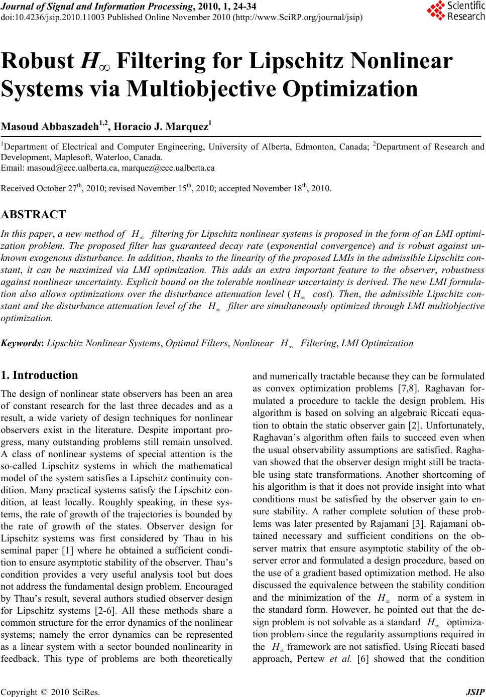Journal of Signal and Information Processing, 20 10 , 1, 24 -34
doi:10.4236/jsip.2010.11003 Published Online November 2010 (http://www.SciRP.org/journal/jsip)
Robust H∞ Filtering for Lipschitz Nonlinear
Systems via Multiobjective Optimization
Masoud Abbaszadeh1,2, Horacio J. Marquez1
1Department of Electrical and Computer Engineering, University of Alberta, Edmonton, Canada; 2Department of Research and
Development, Maplesoft, Waterloo, Canada.
Received October 27th, 2010; revised November 15th, 2010; accepted November 18th, 2010.
ABSTRACT
In this paper, a new method of
H
 filtering for Lipschitz nonlinear systems is proposed in the form of an LMI optimi-
zation problem. The proposed filter has guaranteed decay rate (exponential convergence) and is robust against un-
known exogenous disturbance. In addition, thanks to the linearity of the proposed LMIs in the admissible Lipschitz con-
stant, it can be maximized via LMI optimization. This adds an extra important feature to the observer, robustness
against nonlinear uncertainty. Explicit bound on the tolerable nonlinear uncertainty is derived. The new LMI formula-
tion also allows optimizations over the disturbance attenuation level (
H

cost). Then, the admissible Lipschitz con-
stant and the disturbance attenuation level of the
H

filter are simultaneously optimized through LMI multiobjective
optimization.
Keywords: Lipschitz Nonlinear Systems, Optimal Filters, Nonlinear
H

Filtering, LMI Optimization
1. Introduction
The design of nonlinear state observers has been an area
of constant research for the last three decades and as a
result, a wide variety of design techniques for nonlinear
observers exist in the literature. Despite important pro-
gress, many outstanding problems still remain unsolved.
A class of nonlinear systems of special attention is the
so-called Lipschitz systems in which the mathematical
model of the system satisfies a Lipschitz continuity con-
dition. Many practical systems satisfy the Lipschitz con-
dition, at least locally. Roughly speaking, in these sys-
tems, the rate of growth of the trajectories is bounded by
the rate of growth of the states. Observer design for
Lipschitz systems was first considered by Thau in his
seminal paper [1] where he obtained a sufficient condi-
tion to ensure asymptotic stability of the observer. Thau’s
condition provides a very useful analysis tool but does
not address the fundamental design problem. Encouraged
by Thau’s result, several authors studied observer design
for Lipschitz systems [2-6]. All these methods share a
common structure for the error dynamics of the nonlinear
systems; namely the error dynamics can be represented
as a linear system with a sector bounded nonlinearity in
feedback. This type of problems are both theoretically
and numerically tractable because they can be formulated
as convex optimization problems [7,8]. Raghavan for-
mulated a procedure to tackle the design problem. His
algorithm is based on solving an algebraic Riccati equa-
tion to obtain the static observer gain [2]. Unfortunately,
Raghavan’s algorithm often fails to succeed even when
the usual observability assumptions are satisfied. Ragha-
van showed that the observer design might still be tracta-
ble using state transformations. Another shortcoming of
his algorithm is that it does not provide insight into what
conditions must be satisfied by the observer gain to en-
sure stability. A rather complete solution of these prob-
lems was later presented by Rajamani [3]. Rajamani ob-
tained necessary and sufficient conditions on the ob-
server matrix that ensure asymptotic stability of the ob-
server error and formulated a design procedure, based on
the use of a gradient based optimization method. He also
discussed the equivalence between the stability condition
and the minimization of the
H
 norm of a system in
the standard form. However, he pointed out that the de-
sign problem is not solvable as a standard
H
 optimiza-
tion problem since the regularity assumptions required in
the
H

framework are not satisfied. Using Riccati based
approach, Pertew et al. [6] showed that the condition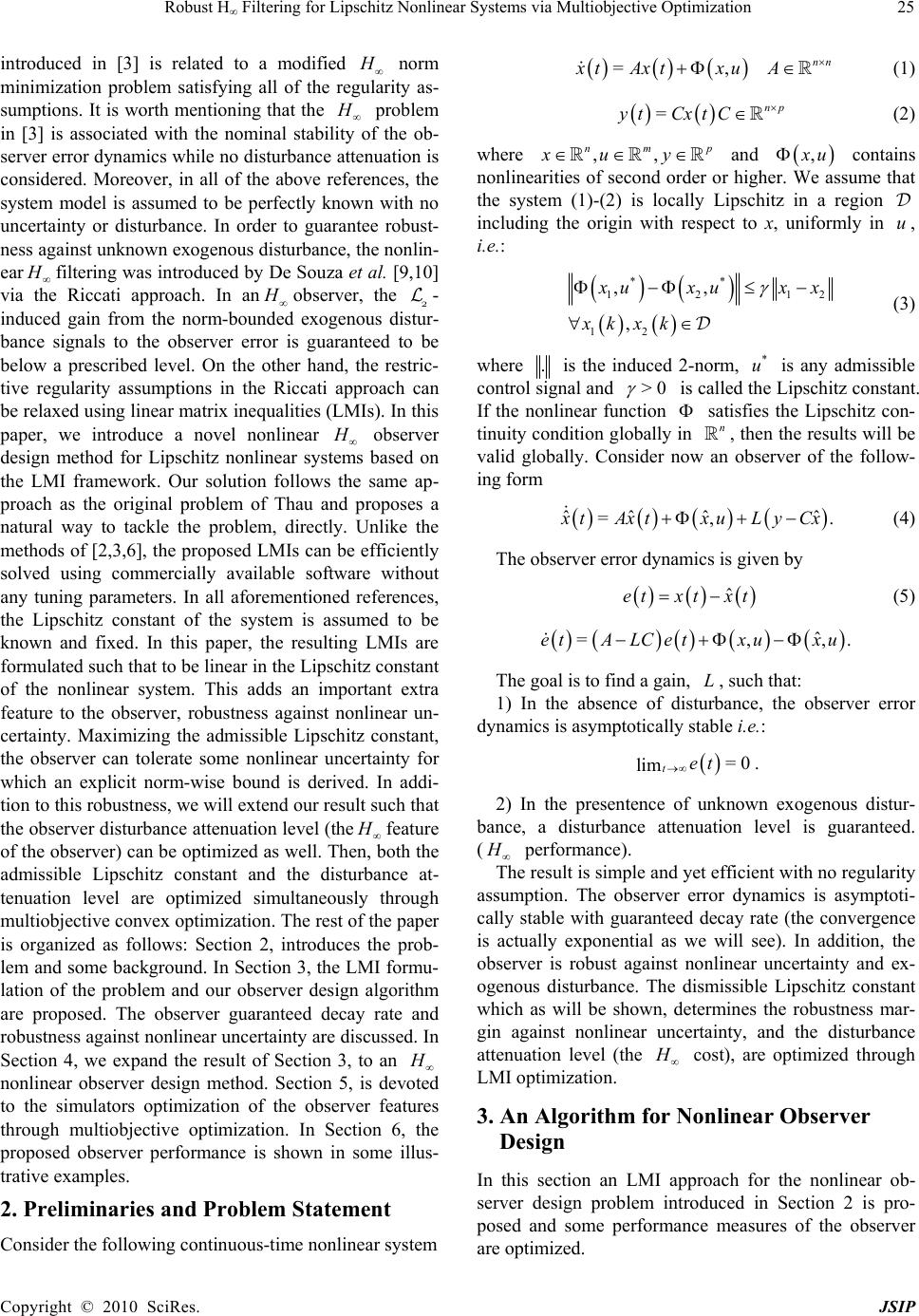

Robust H∞ Filtering for Lipschitz Nonlinear Systems via Multiobjective Optimization
25
introduced in [3] is related to a modified
H

norm
minimization problem satisfying all of the regularity as-
sumptions. It is worth mentioning that the
H
 problem
in [3] is associated with the nominal stability of the ob-
server error dynamics while no disturbance attenuation is
considered. Moreover, in all of the above references, the
system model is assumed to be perfectly known with no
uncertainty or disturbance. In order to guarantee robust-
ness against unknown exogenous disturbance, the nonlin-
ear
H
filtering was introduced by De Souza et al. [9,10]
via the Riccati approach. In an
H
observer, the 
-
induced gain from the norm-bounded exogenous distur-
bance signals to the observer error is guaranteed to be
below a prescribed level. On the other hand, the restric-
tive regularity assumptions in the Riccati approach can
be relaxed using linear matrix inequalities (LMIs). In this
paper, we introduce a novel nonlinear
H
 observer
design method for Lipschitz nonlinear systems based on
the LMI framework. Our solution follows the same ap-
proach as the original problem of Thau and proposes a
natural way to tackle the problem, directly. Unlike the
methods of [2,3,6], the proposed LMIs can be efficiently
solved using commercially available software without
any tuning parameters. In all aforementioned references,
the Lipschitz constant of the system is assumed to be
known and fixed. In this paper, the resulting LMIs are
formulated such that to be linear in the Lipschitz constant
of the nonlinear system. This adds an important extra
feature to the observer, robustness against nonlinear un-
certainty. Maximizing the admissible Lipschitz constant,
the observer can tolerate some nonlinear uncertainty for
which an explicit norm-wise bound is derived. In addi-
tion to this robustness, we will extend our result such that
the observer disturbance attenuation level (the
H

feature
of the observer) can be optimized as well. Then, both the
admissible Lipschitz constant and the disturbance at-
tenuation level are optimized simultaneously through
multiobjective convex optimization. The rest of the paper
is organized as follows: Section 2, introduces the prob-
lem and some background. In Section 3, the LMI formu-
lation of the problem and our observer design algorithm
are proposed. The observer guaranteed decay rate and
robustness against nonlinear uncertainty are discussed. In
Section 4, we expand the result of Section 3, to an
H

nonlinear observer design method. Section 5, is devoted
to the simulators optimization of the observer features
through multiobjective optimization. In Section 6, the
proposed observer performance is shown in some illus-
trative examples.
2. Preliminaries and Problem Statement
Consider the following continuous-time nonlinear system




=,
nn
xtAxtxu A  
 (1)


=np yt CxtC  (2)
where ,,
nm p
xu y   and

,
x
u contains
nonlinearities of second order or higher. We assume that
the system (1)-(2) is locally Lipschitz in a region 
including the origin with respect to x, uniformly in u,
i.e.:




 
**
12 12
12
,,
,
x
uxu xx
xkx k
 


(3)
where . is the induced 2-norm, * u is any admissible
control signal and >0

is called the Lipschitz constant.
If the nonlinear function

satisfies the Lipschitz con-
tinuity condition globally in n , then the results will be
valid globally. Consider now an observer of the follow-
ing form



 
ˆˆ ˆˆ =, .
x
tAxt xuLyCx 
 (4)
The observer error dynamics is given by




ˆ etxt xt (5)






ˆ =,,. etA LCetxuxu 
The goal is to find a gain, L, such that:
1) In the absence of disturbance, the observer error
dynamics is asymptotically stable i.e.:

=0
limtet
 .
2) In the presentence of unknown exogenous distur-
bance, a disturbance attenuation level is guaranteed.
(
H

performance).
The result is simple and yet efficient with no regularity
assumption. The observer error dynamics is asymptoti-
cally stable with guaranteed decay rate (the convergence
is actually exponential as we will see). In addition, the
observer is robust against nonlinear uncertainty and ex-
ogenous disturbance. The dismissible Lipschitz constant
which as will be shown, determines the robustness mar-
gin against nonlinear uncertainty, and the disturbance
attenuation level (the
H

cost), are optimized through
LMI optimization.
3. An Algorithm for Nonlinear Observer
Design
In this section an LMI approach for the nonlinear ob-
server design problem introduced in Section 2 is pro-
posed and some performance measures of the observer
are optimized.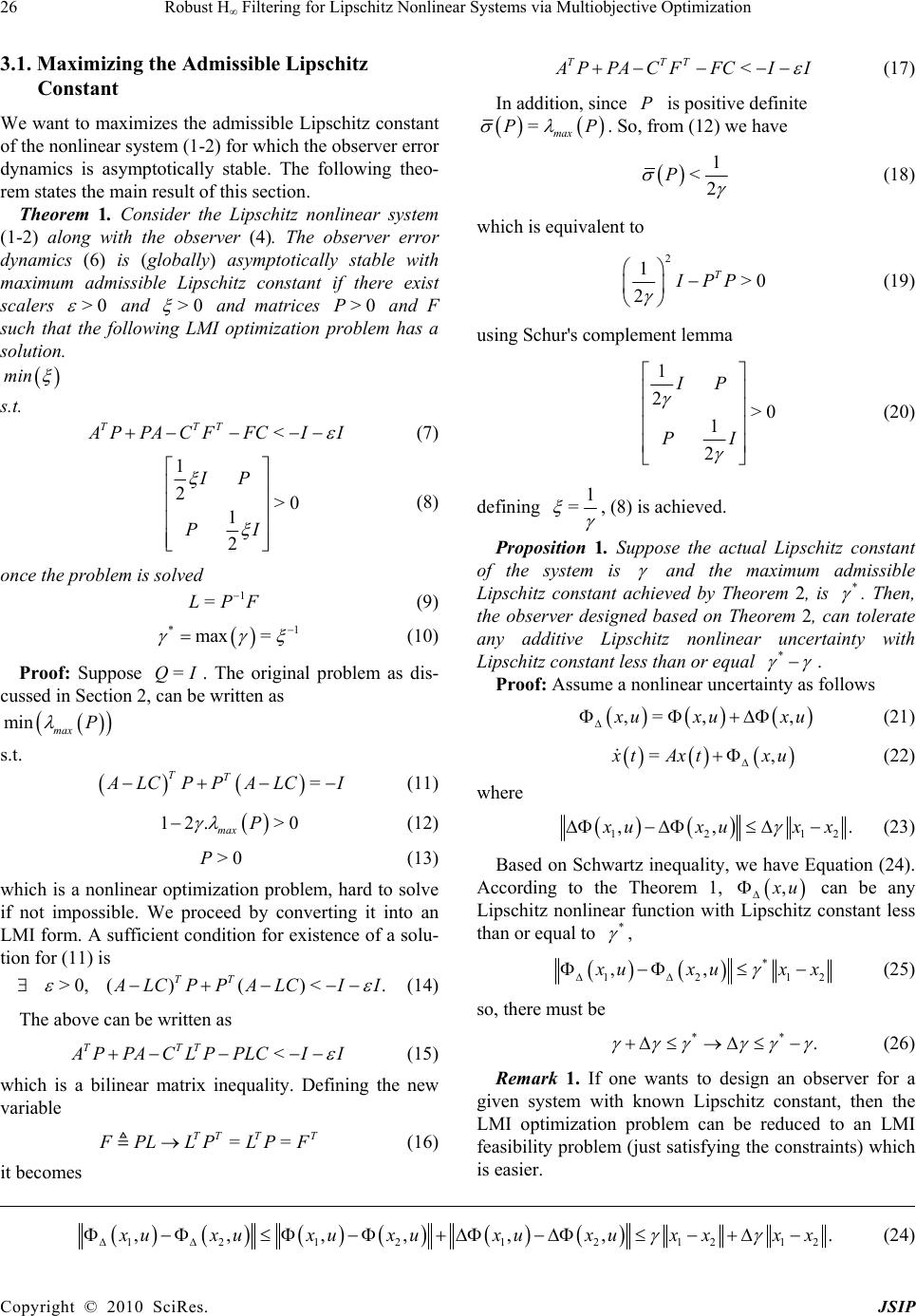

Robust H∞ Filtering for Lipschitz Nonlinear Systems via Multiobjective Optimization
26
3.1. Maximizing the Admissible Lipschitz
Constant
We want to maximizes the admissible Lipschitz constant
of the nonlinear system (1-2) for which the observer error
dynamics is asymptotically stable. The following theo-
rem states the main result of this section.
Theorem 1. Consider the Lipschitz nonlinear system
(1-2) along with the observer (4). The observer error
dynamics (6) is (globally) asymptotically stable with
maximum admissible Lipschitz constant if there exist
scalers >0

and >0

and matrices >0P and F
such that the following LMI optimization problem has a
solution.

min

s.t.
<
TTT
A
PPACFFCI I

  (7)
1
2>0
1
2
IP
PI








(8)
once the problem is solved
1
=LPF
 (9)


*1
max =


 (10)
Proof: Suppose =QI
. The original problem as dis-
cussed in Section 2, can be written as
 
min max P 
s.t.
 
=
TT
A
LCPPA LCI (11)


12. >0
max P
  (12)
>0P (13)
which is a nonlinear optimization problem, hard to solve
if not impossible. We proceed by converting it into an
LMI form. A sufficient condition for existence of a solu-
tion for (11) is
>0,()( )<.
TT
A
LCPPA LCII

  (14)
The above can be written as
<
TTT
A
PPACLPPLCI I

  (15)
which is a bilinear matrix inequality. Defining the new
variable
==
TT TT
F
PLLPLP F (16)
it becomes
<
TTT
A
PPACF FCI I


 (17)
In addition, since P is positive definite




=max PP  . So, from (12) we have

1
<2 P 

(18)
which is equivalent to
2
1>0
2
T
IPP




 (19)
using Schur's complement lemma
1
2>0
1
2
IP
PI








(20)
defining 1 = 

, (8) is achieved.
Proposition 1. Suppose the actual Lipschitz constant
of the system is

and the maximum admissible
Lipschitz constant achieved by Theorem 2, is *

. Then,
the observer designed based on Theorem 2, can tolerate
any additive Lipschitz nonlinear uncertainty with
Lipschitz constant less than or equal *

 .
Proof: Assume a nonlinear uncertainty as follows




,= ,,
x
uxuxu

 (21)




=,
x
tAxt xu


 (22)
where




12 12
,, .
x
uxu xx    (23)
Based on Schwartz inequality, we have Equation (24).
According to the Theorem 1,

,
x
u

 can be any
Lipschitz nonlinear function with Lipschitz constant less
than or equal to *

,




*
1212
,,
x
uxuxx 

 (25)
so, there must be
**
.

 

  (26)
Remark 1. If one wants to design an observer for a
given system with known Lipschitz constant, then the
LMI optimization problem can be reduced to an LMI
feasibility problem (just satisfying the constraints) which
is easier.
 






12121212 12
,,,, ,,.
x
uxuxuxuxuxuxx xx 

 (24)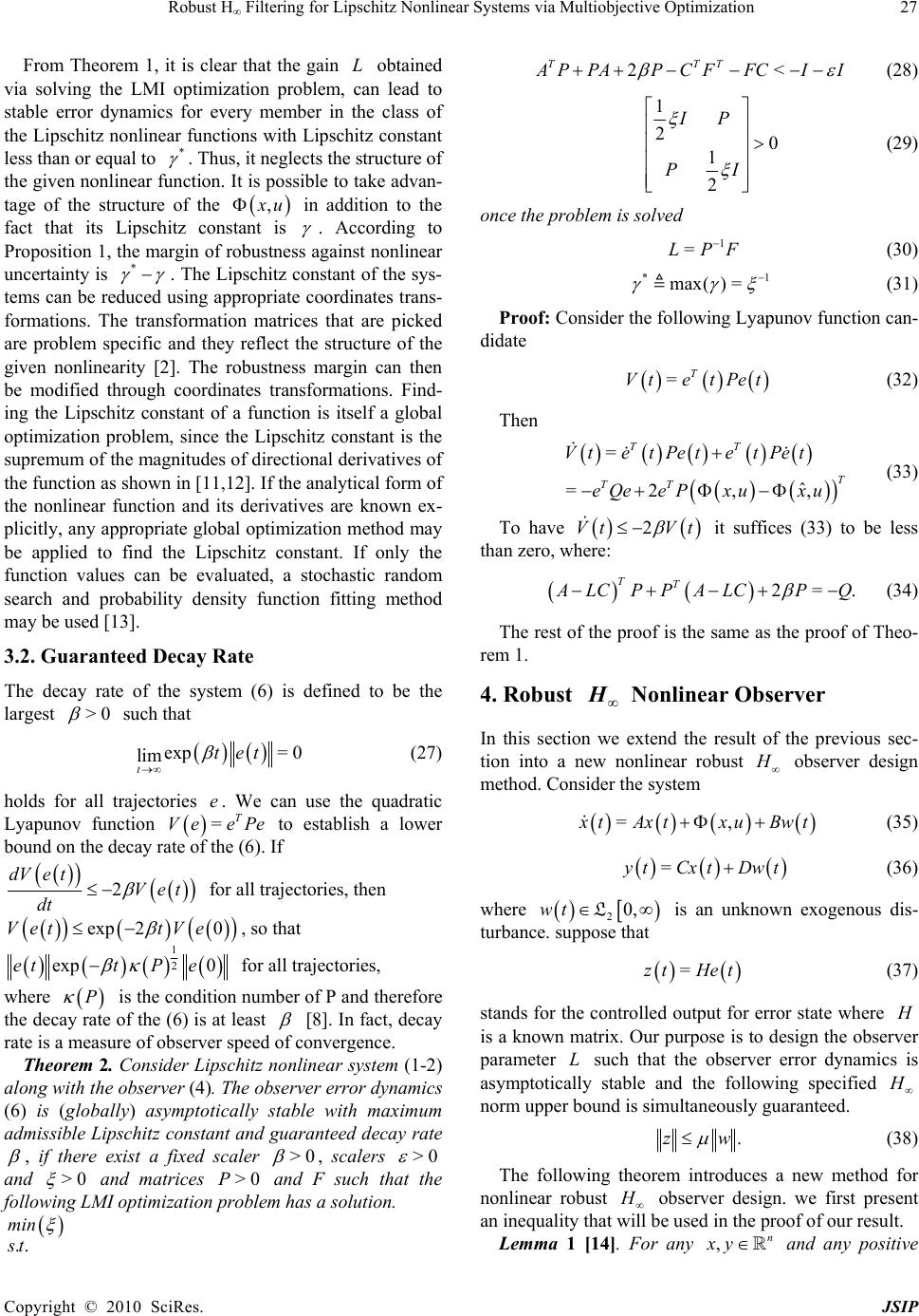

Robust H∞ Filtering for Lipschitz Nonlinear Systems via Multiobjective Optimization
27
From Theorem 1, it is clear that the gain L obtained
via solving the LMI optimization problem, can lead to
stable error dynamics for every member in the class of
the Lipschitz nonlinear functions with Lipschitz constant
less than or equal to *

. Thus, it neglects the structure of
the given nonlinear function. It is possible to take advan-
tage of the structure of the

,
x
u in addition to the
fact that its Lipschitz constant is

. According to
Proposition 1, the margin of robustness against nonlinear
uncertainty is *

 . The Lipschitz constant of the sys-
tems can be reduced using appropriate coordinates trans-
formations. The transformation matrices that are picked
are problem specific and they reflect the structure of the
given nonlinearity [2]. The robustness margin can then
be modified through coordinates transformations. Find-
ing the Lipschitz constant of a function is itself a global
optimization problem, since the Lipschitz constant is the
supremum of the magnitudes of directional derivatives of
the function as shown in [11,12]. If the analytical form of
the nonlinear function and its derivatives are known ex-
plicitly, any appropriate global optimization method may
be applied to find the Lipschitz constant. If only the
function values can be evaluated, a stochastic random
search and probability density function fitting method
may be used [13].
3.2. Guaranteed Decay Rate
The decay rate of the system (6) is defined to be the
largest >0

such that



exp= 0
lim
t
tet 
 (27)
holds for all trajectories e. We can use the quadratic
Lyapunov function

=T Ve ePe to establish a lower
bound on the decay rate of the (6). If


 
2
dVetVet
dt
  for all trajectories, then
   
exp 20Vet tVe   , so that
 
1
2
exp 0ettP e   for all trajectories,
where

P  is the condition number of P and therefore
the decay rate of the (6) is at least

[8]. In fact, decay
rate is a measure of observer speed of convergence.
Theorem 2. Consider Lipschitz nonlinear system (1-2)
along with the observer (4). The observer error dynamics
(6) is (globally) asymptotically stable with maximum
admissible Lipschitz constant and guaranteed decay rate

, if there exist a fixed scaler >0

, scalers >0

and >0

and matrices >0P and F such that the
following LMI optimization problem has a solution.

min

..
s
t
2<
TTT
A
PPAPCFFCI I



  (28)
1
20
1
2
IP
PI




 



(29)
once the problem is solved
1
=LPF
 (30)
*1
max()=



 (31)
Proof: Consider the following Lyapunov function can-
didate


=T Vte tPet (32)
Then






  
=
ˆ =2,,
TT
T
TT
Vte tPete tPet
eQeePxuxu



(33)
To have




2Vt Vt  
 it suffices (33) to be less
than zero, where:
 
2=.
TT
A
LCPPA LCPQ 

 (34)
The rest of the proof is the same as the proof of Theo-
rem 1.
4. Robust

H
Nonlinear Observer
In this section we extend the result of the previous sec-
tion into a new nonlinear robust
H
 observer design
method. Consider the system



 
=,
x
tAxt xuBwt 
 (35)


=
y
tCxtDwt (36)
where




20,wt

L is an unknown exogenous dis-
turbance. suppose that


=zt Het (37)
stands for the controlled output for error state where
H
is a known matrix. Our purpose is to design the observer
parameter L such that the observer error dynamics is
asymptotically stable and the following specified
H

norm upper bound is simultaneously guaranteed.
.zw   (38)
The following theorem introduces a new method for
nonlinear robust
H

observer design. we first present
an inequality that will be used in the proof of our result.
Lemma 1 [14]. For any ,n
xy and any positive

Robust H∞ Filtering for Lipschitz Nonlinear Systems via Multiobjective Optimization
28
definite matrix nn P , we have
1
2TT T
x
yxPxyPy

 (39)
Theorem 3. Consider the Lipschitz nonlinear system
(35-36) with given Lipschitz constant

, along with the
observer (4). The observer error dynamics is (globally)
asymptotically stable with decay rate

and minimum
2()weL gain,

, if there exist fixed scaler >0

,
scalers >1

, >0

and >0

and matrices >0P
and
F
such that the following LMI optimization prob-
lem has a solution.

min

s.t.
2<
TTT
A
PPAPCFFCII

   (40)


2
2
1
2>0
1
2
HIP
H
PI













(41)
11
2<0
2
T
TTT
HHIPB FD
BP DFI













(42)
Once the problem is solved
1
=LPF
 (43)

*min =



 (44)
Proof: The observer error dynamics will be







 
ˆ
=,,etA LCetxuxuBLDw

(45)
consider the following Lyapunov function candidate


=T Vte tPet (46)
then






  


=
ˆ
=2,,
TT
T
TT
TTTTT
Vte tPete tPet
eQeePxuxu
e PBFDwwBPDFe




(47)
where, Q is as in (34). We select =QI

. If =0w
the error dynamics is as Theorem 2, so the LMIs (7) and
(8) which for =QI

will become
2<
TTT
A
PPAPCF FCI I



  (48)
2>0
2
IP
PI










(49)
are sufficient for the asymptotic stability of the error dy-
namics. Having >1

, (18) always implies (49).
Based on Rayleigh inequality

TT
max
eQe Qee   (50)
Using Lemma 1 we can write
        
     
1
ˆˆˆ 2(,,,, ,,
ˆˆ =,,,,
T
TT
T
T
ePxu xuePe xu xuPPPxuxu
ePexu xuPxu xu


   (51)
based on Rayleigh inequality we have
 
2=
TT
max max
ePeP ePee   (52)
       
22
22
ˆˆ ˆ
,, ,,,,=
TT
maxmax max
x
u xuPxu xuPxu xuPePee     (53)
therefore, from the above and (18),
  


211
ˆ 2,,1 .
2
TTT
max
eP xuxuPeeee  

 


(54)
According to (50) and (54) and knowing that =QI

, we have
 

11
2.
2
TTTT TT
VteeePBFDw wBP DFe 


 


 (55)
Now, we define

0
=TT
J
zz wwdt 

 (56)
therefore


0
<TT
J
zzww Vdt 

 (57)

Robust H∞ Filtering for Lipschitz Nonlinear Systems via Multiobjective Optimization
29
it follows that a sufficient condition for 0J is that


0, ,0
TT
tzzwwV   
 (58)
but we have Equation (59).
Thus, a sufficient condition for 0J is that the
above matrix which is the same as (42) be negative defi-
nite. Then
0
TT
zz wwzw   (60)
Up until now, we have the LMIs (48), (20) and (42). If
these LMIs are all feasible, then the problem is solvable
and the observer synthesis is complete. However, (20)
can be slightly modified to improve its feasibility. We
proceed as follows:
Inequality (51) can be rewritten as follows
   
ˆ
2,,2
TT
max
eP xuxuPee    (61)
following the same steps, the matrix in (59) will become

[2 ]<0.
T
max
TTT
H HPIPBFD
BP DFI
 






(62)
The above matrix can not be used together with (48)
and (49) because it includes P as one of the LMI vari-
ables, thus resulting in a problem that is not linear in P.
It can, however, give us another insight about


max P
 .
According to the Schur's complement lemma, (62) is
equivalent to
<0I

 (63)
 
1
2<0.
T
T
max
HHPIPB FD PB FD   

(64)
The third term in the above is always nonnegative, so
it is necessary to have


[2]< 0
T
max
HHPI    (65)
but as for any other symmetric matrix, for T
HH
, we
have
 
TT T
min max
H
HI HHHHI   (66)
or according to the definition of singular values


22
T
H
IHH HI   (67)
therefore, a sufficient condition for (65) is


22<0
max
HP   (68)
or
 
2
<2
max
H
P


 (69)
but (18) must be also satisfied. To have both (18) and
(69), it is sufficient that
 
2
1
<2
max
H
P


 (70)
which is equivalent to (41).
Remark 2. Similar to Remark 1, if one wants to design
an observer for a given system with known Lipschitz
constant and with a prespecified

, the LMI optimiza-
tion problem is reduced to an LMI feasibility problem.
Remark 3. As an additional opportunity, we can first
maximize the admissible Lipschitz constant using Theo-
rem 3, and then minimize

for the maximized

,
using Theorem 3. In this case, according to Proposition 1,
robustness against nonlinear uncertainty is also guaran-
teed. In the next section, we will show that how

and

can be simultaneously optimized using convex mul-
tiobjective optimization. It is clear that if no decay rate is
specified, then the term 2P

will be eliminated from
LMI (40) in Theorem 3.
5. Combined Performance using
Multiobjective Optimization
The LMIs proposed in Theorem 3 are linear in both ad-
missible Lipschitz constant and disturbance attenuation
level and as mentioned earlier, each can be optimized. A
more realistic problem is to choose the observer gain
matrix by combining these two performance measures.
This leads to a Pareto multiobjective optimization in
which the optimal point is a trade-off between two or
more linearly combined optimality criterions. Having a
fixed decay rate, the optimization is over

(maximiza-
tion) and

(minimization), simultaneously. The


11
2
2
11
2
2
=.
TTTTTTTT
T
T
TTTTTT
TTT
zzww VeHHewwVeHHeee
HHIPB FD
ee
e PBFDwwBPDFewwww
BP DFI







 











 





 



(59)

Robust H∞ Filtering for Lipschitz Nonlinear Systems via Multiobjective Optimization
30
following theorem is in fact a generalization of the re-
sults of [2-6, 15], and [9] (for systems of class (1-2)) in
which the Lipschitz constant is assumed to be known and
fixed and the result of [7] in which a special class of sec-
tor nonlinearities is considered.
Theorem 4. Consider the Lipschitz nonlinear system
(35-36) along with the observer (4). The observer error
dynamics is (globally) asymptotically stable with decay
rate

and simultaneously maximized admissible
Lipschitz constant

and minimized

2weL gain,.

, if there exist fixed scalers 01

 and >0

,
scalers >1

, >0

, >0

and >0

and matrices
>0P and
F
such that the following LMI optimization
problem has a solution


1min



 

s.t.
2<
TTT
A
PPAPCF FCI I

   (71)


2
2
1
2>0
1
2
HIP
H
PI










(72)

12
2
20<0
0
T
TTT
HHIIPB FD
II
BP DFI




 










(73)
Once the problem is solved,
1
=LPF
 (74)
*1
max()=



 (75)
*min() =



 (76)
Proof: The above is a scalarization of a multiobjective
optimization with two optimality criteria. Since each of
these optimization problems is convex, the scalarized
problem is also convex [16]. The rest of the proof is the
same as the proof of Theorem 3 where the LMI (73) is
obtained from the LMI (42) using the Schur’s comple-
ment lemma.
6. Illustrative Examples
In this section the high performance of the proposed ob-
server is shown via three design examples.
Example 1. Consider the following observable (A,C)
pair

01
=,=01
11
AC




The result of the iterative algorithm proposed in [38] is
*=0.49


=69.552311.5679 T L
while using our proposed method in Theorem 1,
*=1.1933


=56.833421.9074 T L
which means that the admissible Lipschitz constant is
improved by a factor of 2.42 .
Example 2. The following system is the unforced
forth-order model of a flexible joint robotic arm as pre-
sented in [2,4,5]. The reason we have chosen this exam-
ple is that it is an important industrial application and has
been widely used as a benchmark system to evaluate the
performance of the observers designed for Lipschitz
nonlinear systems.
0100 0
48.61.25 48.6 00
=0001 0
19.5019.503.33sin(3)
xx
x

 

 


 


 

 


 

1000
=.
0100
yx






The system is globally Lipschitz with Lipschitz con-
stant =3.33

. Noticing the structure of  that has a
zero entry in three of its channels, Raghavan [2], pro-
posed the coordinates transformation =
x
Tx , where


=1,1,4,0.1Tdiag under which the transformed sys-
tem has Lipschitz constant =0.083

. Using Theorem 2,
*=0.4472
 in the original coordinates and *= 2.4177 
in the transformed coordinates. The observer gain L, is
obtained in the transformed coordinates and computed in
the original coordinates as 1 =LTL
. Assuming
=0.2

,

=1111
T
B,

=0.10.25T D,
44
=0.5 ,
H
I
and using Theorem 3 we get, *=0.5753
 , =2.0517

,
= 0.0609

, and finally the observer gain will be
33.4865129.924959.89713 108.2134
=.
38.5694282.8603102.1561 171.0910
T
L






Figure 1, shows the true and estimated values of states.
The actual states are shown along with the estimates ob-
tained using Raghavan's [2] and Aboky's [5] methods and
our proposed LMI optimization method. The initial con-

Robust H∞ Filtering for Lipschitz Nonlinear Systems via Multiobjective Optimization
31
Figure 1. The true and estimated states of Example 2.
ditions for the system are
 
0=01 02
T
x and
those of the all observers are
 
ˆ0=1 00.50
T
x.
As seen in Figure 1, the observer designed using the
proposed LMI optimization method has the best conver-
gence of the three. Note that in addition to the better
convergence, the proposed observer is an
H

filter
with maximized disturbance attenuation level while the
observers designed based on the methods of [2-6] can
only guarantee stability of the observer error.
Example 3. In this example we show the usage of the
multiobjective optimization of Theorem 4 in the design
of
H
observers. Consider the following system

12
=T
x
xx
3
1
52 42
11211
01
=11 66 22
x
xx
x
xx xx




  





=1 0.
y
x
The systems is locally Lipschitz. Its Lipschitz constant
is region-based. Suppose we consider the region  as
follows


2
12 1
= ,0.25xx x
in which the Lipschitz constant is =0.4167

. We
choose
=0.5
H
I,

=1 1
T
B,=0.2D,=0.05

and solve the multiobjective optimization problem of
Theorem 4 with =0.9

. We get
*=0.5525

*= 1.1705

= 1.6260

4
= 2.243510 



= 23.702513.7272.
T
L
The true and estimated values of states are
shown in Figure 2. We have assumed that


0= 0.21.45
T
x
 
ˆ0=0.252 T
x



=0.15expsin .wtt t
For any

  
20,wt

L, disturbance rejec-
tion ratio

should be less than or equal 0.3371 (ob-
tained for =0

). The actual disturbance rejection ratio
of this simulation is 0.2302. If instead, =0.5

then
*=0.4686
 , =1.4161

, = 0.0067


=329.9735244.1398 T L
Since the observer gain directly amplifies the measure-

Robust H∞ Filtering for Lipschitz Nonlinear Systems via Multiobjective Optimization
32
Figure 2. The true and estimated states of Example 3 in the presence of disturbance.
Figure 3. *

, *

and ()
L

, and the optimal trade-off curve with =0.05

.

Robust H∞ Filtering for Lipschitz Nonlinear Systems via Multiobjective Optimization
33
Figure 4. The optimal surface of *

.
Figure 5. The optimal surface of*

.
ment noise, sometimes, it is better to have an observer
gain with smaller elements. There might also be practical
difficulties in implementing high gains. We can control
the Frobenius norm of L either by changing the feasi-
bility radius of the LMI solver or by decreasing


1
min P


which is


1
max P

, to decrease


L  . The latter can
be done by replacing >0P with >PI

in which
>0

can be either a fixed scaler or an LMI variable.
Using these tricks, an observer with the same decay ratio
=0.5

but much smaller Frobenius norm of gain, can

Robust H∞ Filtering for Lipschitz Nonlinear Systems via Multiobjective Optimization
34
be achieved
*=0.5314
 , = 1.3973

, = 0.0125


=134.404090.0881T L
as seen, the price of this is bigger disturbance rejection
ratio. The values of *

, *

, norm of the observer gain
matrix, ()L

, and the optimal trade-off curve between
*

and *

over the range of

when the decay rate
is fixed

=0.05  are shown in Figure 3. As seen in
the figure, there is a trade of between the Lipschitz
maximization (the robustness feature against nonlinear
uncertainty) and the disturbance attenuation (the
H

performance). We like to have a *

as large as possible
and a *

as small as possible. The parameter that con-
trols this trade off is the weight

used in the cost
function of the proposed Pareto convex optimization.
Pareto multiobjective optimization leads to an optimal
curve rather than a single point. The selection of particu-
lar point on that curve is then based on the appropriate
selection of

based on the acceptable values for *

and *

.
The values of *

, *

, norm of the observer gain ma-
trix, ()L

, and the optimal trade-off curve between *

and *

over the range of

when the decay rate is
fixed

=0.05  are shown in Figure 3. The optimal
surfaces of *

and *

over the range of

when the
decay rate is variable are shown in Figures 4,5, respec-
tively.
7. Conclusions
A new method of robust observer design for Lipschitz
nonlinear systems proposed based on LMI optimization.
The Lipschitz constant of the nonlinear system can be
maximized so that the observer error dynamics not only
be asymptotically stable but also the observer can toler-
ate some additive nonlinear uncertainty. In addition, the
result extended to a robust
H

nonlinear observer. The
obtained observer has three features, simultaneously.
Asymptotic stability, robustness against nonlinear uncer-
tainty and minimized guaranteed
H
 cost. Thanks to
the linearity of the proposed LMIs in both admissible
Lipschitz constant and the disturbance attenuation level,
they can be simultaneously optimized through convex
multiobjective optimization. The observer high perform-
ance showed through design examples.
REFERENCES
[1] F. Thau, “Observing the State of Nonlinear Dynamic
Systems,” International Journal of Control, Vol. 17, No.
3, 1973, pp. 471-479.
[2] S. Raghavan and K. J. Hedrick, “Observer Design for a
Class of Nonlinear Systems,” International Journal of
Control, Vol. 59, No. 2, 1994, pp. 515-528.
[3] R. Rajamani, “Observers for Lipschitz Nonlinear Sys-
tems,” IEEE Transactions on Automatic Control, Vol. 43,
No. 3, 1998, pp. 397-401.
[4] R. Rajamani and Y. M. Cho, “Existence and Design of
Observers for Nonlinear Systems: Relation to Distance to
Unobservability,” International Journal of Control, Vol.
69, No. 5, 1998, pp. 717-731.
[5] C. Aboky, G. Sallet and I. C. Walda, “Observers for
Lipschitz Non-Linear Systems,” International Journal of
Control, Vol. 75, No. 3, 2002, pp. 534-537.
[6] A. Pertew, H. J. Marquez and Q. Zhao, “H∞ Observer
Design for Lipschitz Nonlinear Systems,” IEEE Transac-
tions on Automatic Control, Vol. 51, No. 7, 2006, pp.
1211-1216.
[7] A. Howell and J. K. Hedrick, “Nonlinear Observer De-
sign via Convex Optimization,” Proceedings of the Ame-
rican Control Conference, Vol. 3, 2002, pp. 2088-2093.
[8] S. Boyd, L. E. Ghaoui, E. Feron and V. Balakrishnan,
“Linear Matrix Inequalities in System and Control The-
ory,” Society for Industrial and Applied Mathematics,
Philadelphia, 1994.
[9] C. E. de Souza, L. Xie and Y. Wang, “H∞ Filtering for a
Class of Uncertain Nonlinear Systems,” Systems and
Control Letters, Vol. 20, No. 6, 1993, pp. 419-426.
[10] Y. Wang, L. Xie and C. E. de Souza, “Robust control of a
class of uncertain nonlinear systems,” Systems and Con-
trol Letters, Vol. 19, No. 2, 1992, pp. 139-149.
[11] H. Khalil, “Nonlinear Control Systems,” 3rd Edition,
Prentice Hall, Upper Saddle River, New Jersey, 2002.
[12] H. J. Marquez, “Nonlinear Control Systems: Analysis and
Design,” Wiley, New York, 2003.
[13] G. Wood and P. Zhang, “Estimation of the Lipschitz con-
stant of a function,” Journal of Global Optimization, Vol.
8, No. 1, 1996, pp. 91-103.
[14] S. Xu, “Robust H∞ Filtering for a Class of Discrete-Time
Uncertain Nonlinear Systems with State Delay,” IEEE
Transactions on Circuits and Systems I: Fundamental
Theory and Applications, Vol. 49, No. 12, 2002, pp.
1853-1859.
[15] F. Zhu and Z. Han, “A Note on Observers for Lipschitz
Nonlinear Systems,” IEEE Transactions on Automatic
Control, Vol. 47, No. 10, 2002, pp. 1751-1754.
[16] S. Boyd and L. Vandenberghe, “Convex Optimization,”
Cambridge University Press, 2004.