Applied Mathematics
Vol.3 No.10A(2012), Article ID:24116,9 pages DOI:10.4236/am.2012.330209
An Implementation Method for the Geodesics with Constraints on Heisenberg Manifolds
Department of Mathematics, Institute of Sciences, Setif, Algeria
Email: khellafyasmina@yahoo.fr
Received July 10, 2012; revised August 30, 2012; accepted September 7, 2012
Keywords: Christoffel; Metric; Heisenberg; Geodesic; Levi-Civita
ABSTRACT
In this paper we address the implementation issue of the geodesics method with constraints on Heisenberg manifolds. First we present more details on the method in order to facilitate its implementation and second we consider Mathematica as a software tool for the simulation. This implementation is of great importance since it allows easy and direct determination of Ricci tensor, which plays a fundamental role in the Heisenberg manifold metric.
1. Introduction
Geodesics plays an important role in many applications, especially in nuclear physics, image processing, ··· Ovidiu Calin and Vittorio Mangione [1] considered the Heisenberg manifold structure to provide a qualitative characterization for geodesics under nonholonomic constraints. This method offers an excellent description or the solution of Euler—Lagrange equation associated to lagrangians with linear and quadratic constraints. Therefore it is highly desirable to consider the implementation of this interesting mathematical method. In this paper we investigate the implementation of the method presented in reference [1]. Due to the fact that the mathematical work in reference [1] lacks some details that are necessary for implementation, we address this issue by including such required details with complete proofs, after presenting the method described elsewhere [1] in an appropriate manner we implement and simulate mathematical. This implementation approach can successfully well illustrate the variation of some parameters such as Christoffel coefficients, ··· and ··· that are required in the determination of tensors. Our approach is also of great importance especially in the case where the determination of the geodesics is carried out by minimizing a performance index. Therefore our implementation approach can be considered as an attractive complement for the work of [1].
The working hypotheses:
We take the examples studied in [1] with the following:
1) Expressions of the vector fields
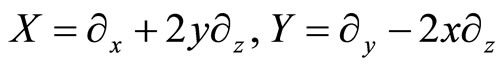 (1)
(1)
2) The Heisenberg Laplacian operator
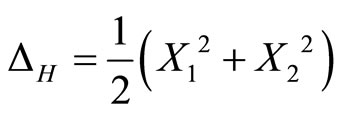 (2)
(2)
3) The sub-Riemannian geometry can be defined on  by:
by:
 (3)
(3)
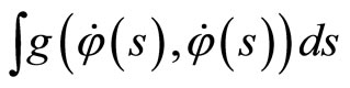
4) If  is the trajectory of a particle of mass m = 1 its energy is given by
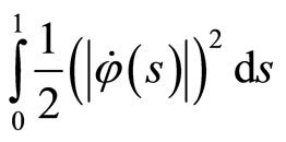 (4)
(4)
where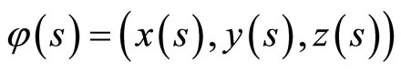 , and
, and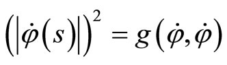 is a Riemannian metric which will be specified later.
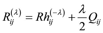
5) We consider successively the two expressions:
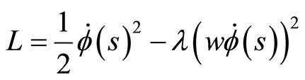 (5)
(5)
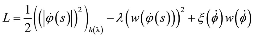
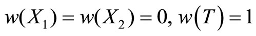
where w is the 1-form such
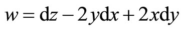
And  is a constant, which has the physical significance of a charge.
  is a 1-form which will be defined later.
6) We consider as in [2], the Heisenberg group
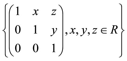
This group is non commutative and the law of the group is polynomial and can be written in 

The Lie algebra of H is spanned by the matrices
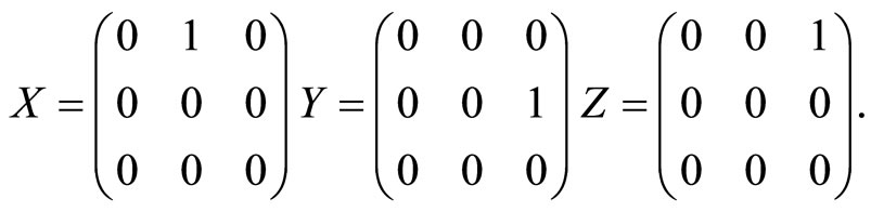
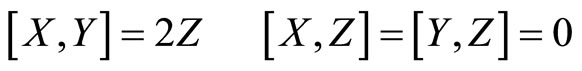
for which the following relations hold
Proposition:
If A and B are in H,
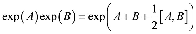
This relation is not so senseless even if it can be very easily proved with a little computation.
It is indeed coming from the Baker-Campb-Hausdorff formula which expresses the product of the exponential of two matrices as the exponential of some quantity.
To be more precise, for two matrices M and N:
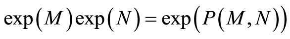
where  is a Lie series which depends on the iterated brackets of M and N:
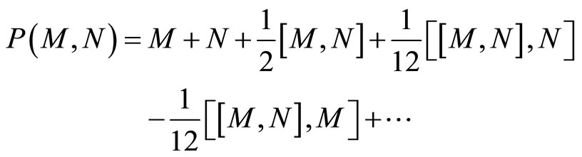
In this case of the Heisenberg group whose Lie algebra is nilpotent of order 2, this serie stops after the first bracket term. We prefer to work with the exponential coordinates are the coordinates in the Lie algebra.
We identify  then with the triple
  such that:
The group law in these coordinates becomes:

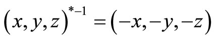
And the inverse element is:
The expressions of the left invariant vector fields in these exponential coordinates are then
 (6)
(6)
Whereas the right-invariant vector fields is written:
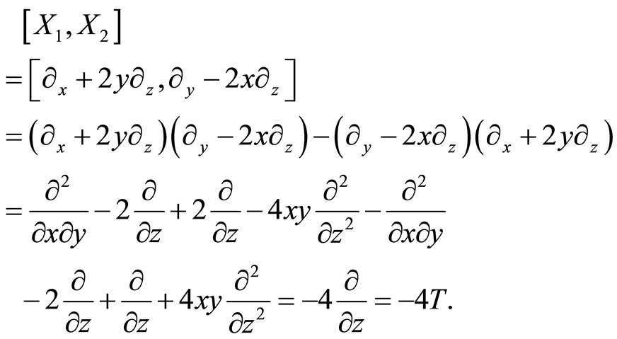
Reference [3] was the first to check easily that:
 (7)
(7)
And
The left invariant frame ,
,  is a basis for the horizontal fibration
Note that
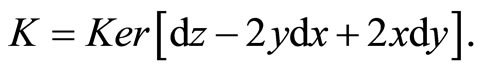
 (8)
(8)
Is a contact form in  i.e.
i.e. 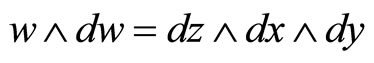 (
( never vanishes); since
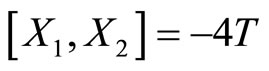 , it follows that K is not involutive.The distribution K will be called the horizontal distribution.
A more detailed about sub-Riemannian structures see in [4].
A curve  is called horizontal if
Or
 (9)
(9)
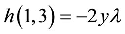
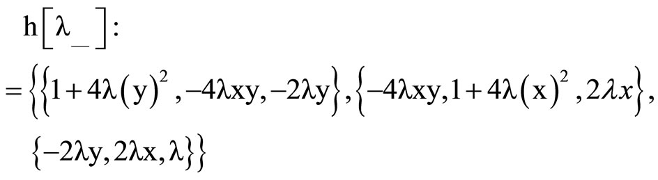
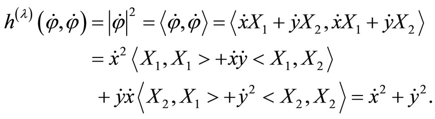
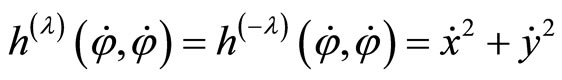
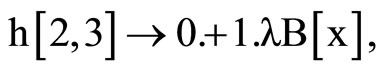
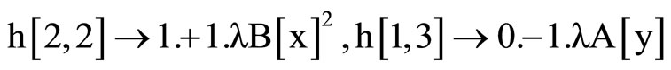
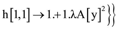
The vector fields (6) defines a unique Riemannian metric h such as
And  .
.
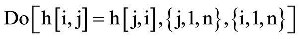
For the coefficients calculus, we have used a little Mathematica program:


 So, we have :
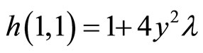 ,
, 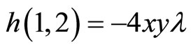 ,
, 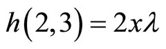 ,
,
 ,
,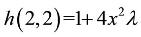
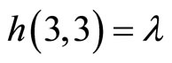 .
.
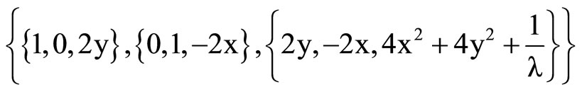
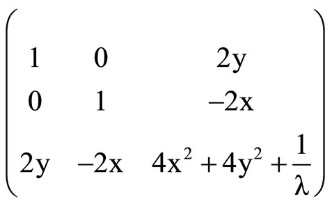
As the coefficients  are symmetric in i and j the matrix of coefficients is
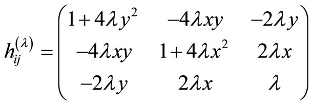 (10)
(10)
For a detailed study of sub-Riemannian geodesics on Heisenbeg group see in [5].
2. Main Results [6]
Heisenberg group case:
We shall construct the Euler-Lagrange equation for the Lagrangian (5) in the Levi-Civita connection form.
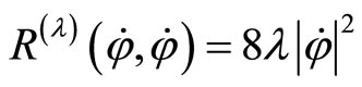
Lemma 1
If  are the components of the Ricci tensor with respect to the metric
  on
on  then
then
 (11)
(11)
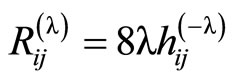
Proof
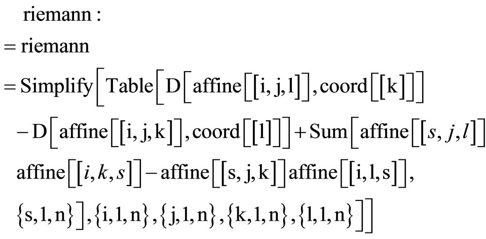
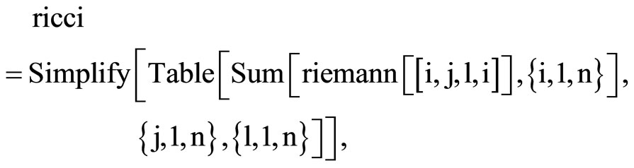
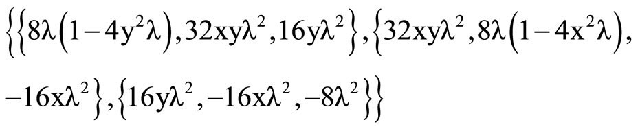
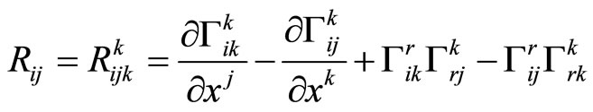
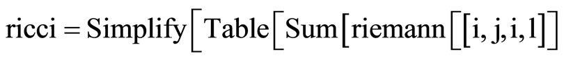
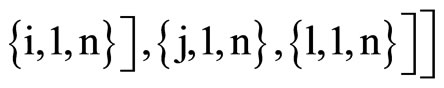
We will calculate the coefficients of the Ricci tensor from the following relation:

After, we will compare these results with those of theorem.
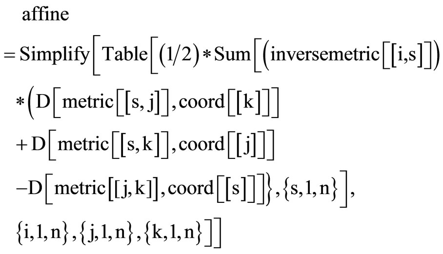
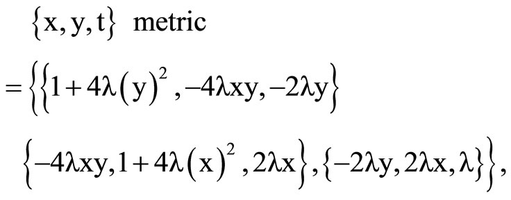
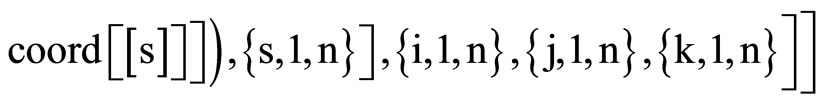
For the first calculation, we use the mathematica program:
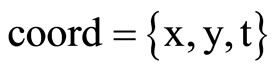
Clear [coord, metric, inversemetric, affine, riemann, ricci,scalar, x, y, t]

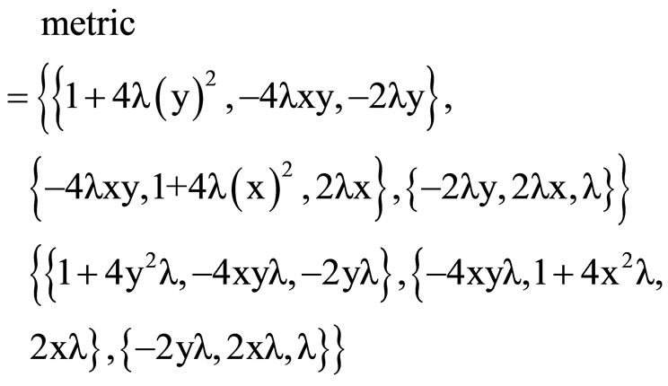
Metric // MatrixForm
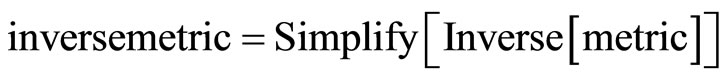
Imversemetric = Simplify [Inverse [metric]]
inversemetric // MatrixForm
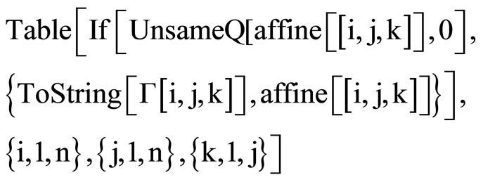
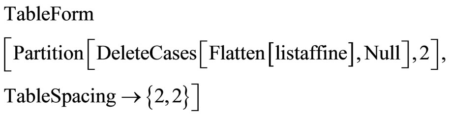
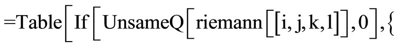
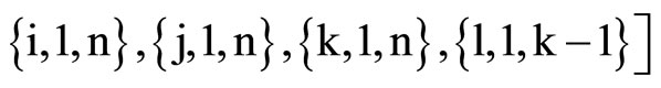
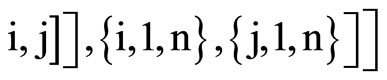
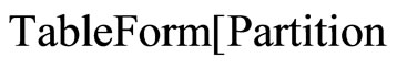
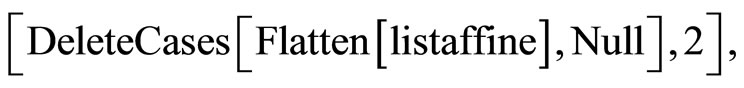
TableForm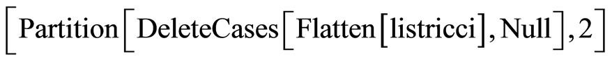 ,
,
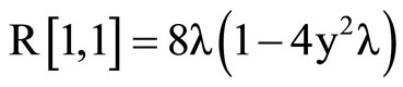
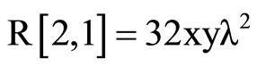
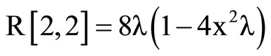
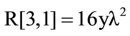
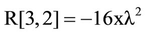
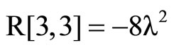
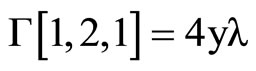
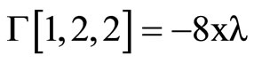
LikewiseUsing (10) where we swap  with
with  , we get the Equation (11) on components:
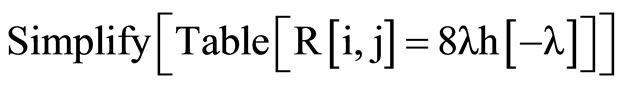
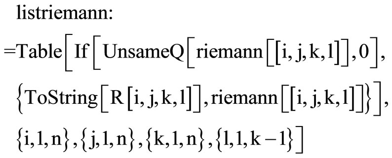
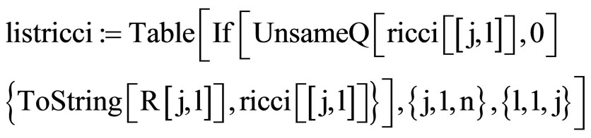
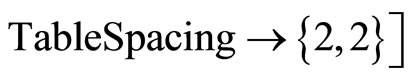
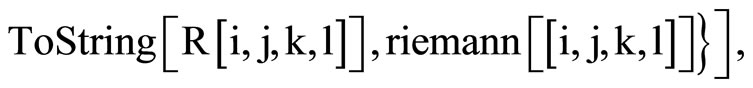
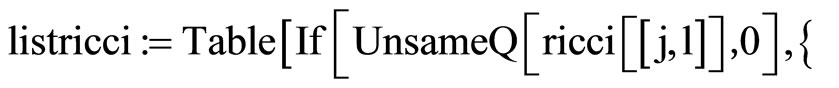
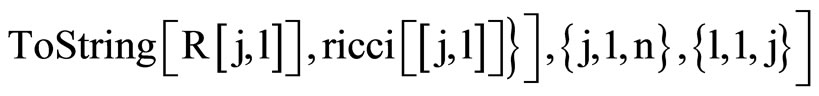
Remarque:
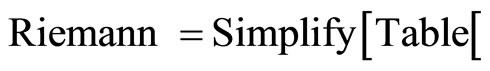
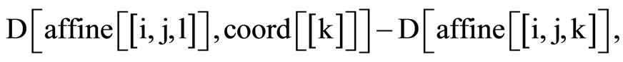
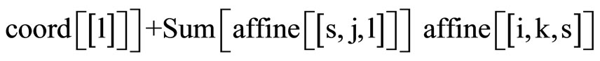
To show the values of the Riemann tensor, add the following command :
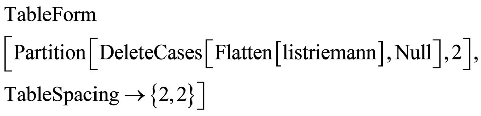
Corollary 1
If  is an horizontal curve ,then
 (12)
(12)
where 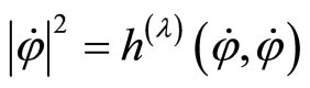 does not depend on
Proof If  is horizontal,
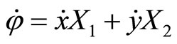 . In this case,
so we have
We see that  does not depend on
  .
.
Using lemma1:
The next proposition is a generalization of the previous corollary to any vector field.
Proposition 1
For any vector field V we have
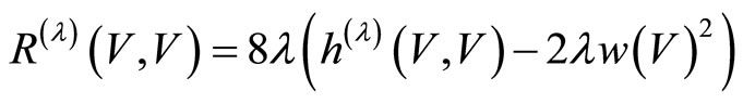 (13)
(13)
Proof Using the metric , we can write
 (14)
(14)
where
we have
And (14) becomes
Using lemma1:
Corollary 2
The actions 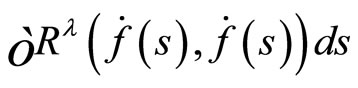 and
and 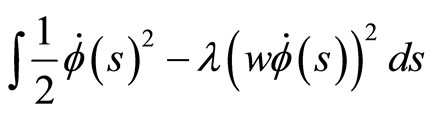 both with respect to the metric
 reach the extrema for the same functions
  .
.
In particular, the extrema will be geodesics in the metric with coefficients .
.
It is interesting that, even if the Lagrangian (5) has a non-holonomic constraint, the minimizers still behave as geodesics in a certain metric. This is given in the following result.
Theorem 1
The Euler-Lagrange equation for the Lagrangian (5) is
 (15)
(15)
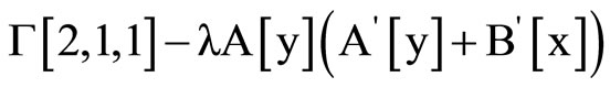
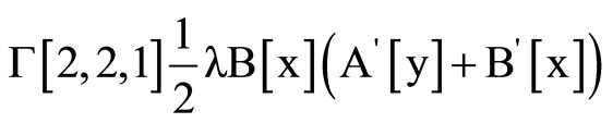
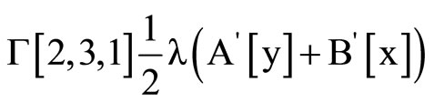
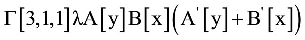
where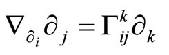 , with the coefficients given by
 (16)
(16)
3. A More General Case [6]
Heisenberg manifold case
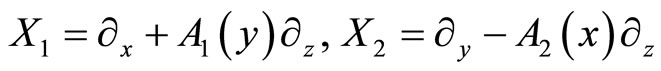
We have investigated the case when the vector fields are given by the formula (3). We shall deal in this section with the more general case of vector fields.
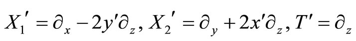
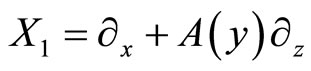 And
And 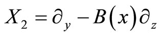
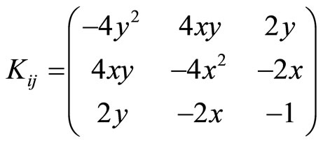
With A(y), B(x) are smooth functions. The 1-form w in this case is
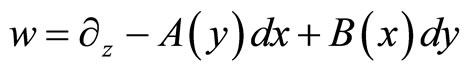 (17)
(17)
One may check that
 (18)
(18)
Another important 1-form is
 (19)
(19)
A computation shows the vector fields ,
,  and
and  are orthonormal in the Riemannian metric.
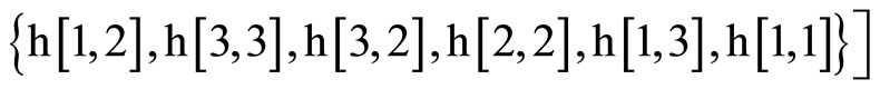
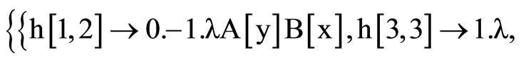
For computing the coefficients, we have use a little Mathematica program.

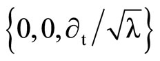

NSolve


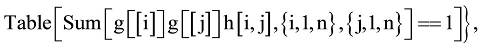

 ,
,
So, we have:
 ,
, 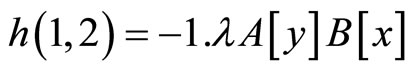
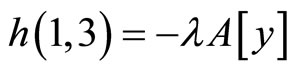 ,
,
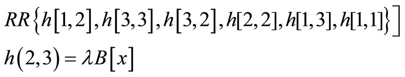
 ,
,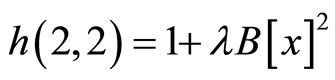 .
.
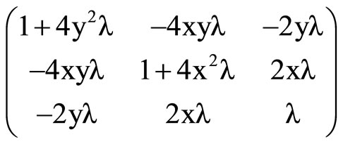
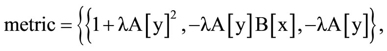
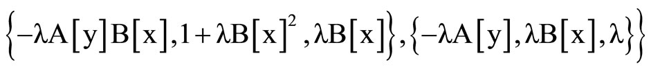
As the Riemannian metric is symmetric, we obtain
 (20)
(20)
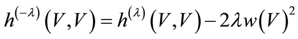
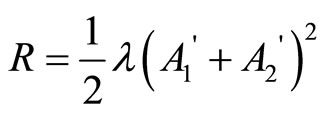
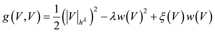
We shall consider the following Lagrangian with a quadratic potential constraint
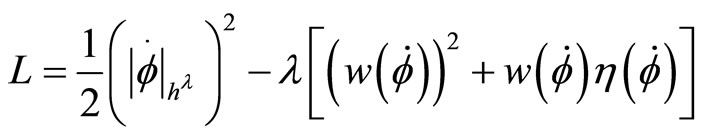 (21)
(21)
When  and
and  we get the Lagrangian in (5). In this case
 .
.
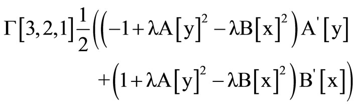
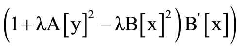
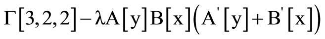
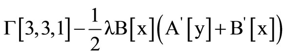
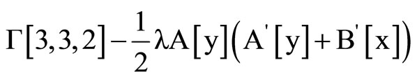
The following result is a generalization of lemma1.We shall denote by
 ,
, (22)
(22)
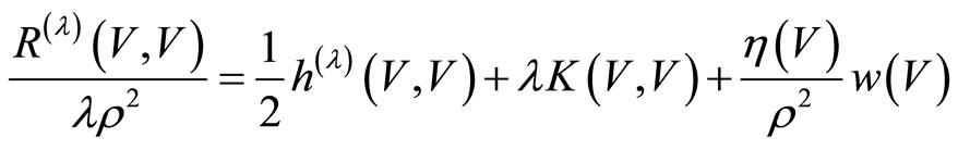
Lemma 2
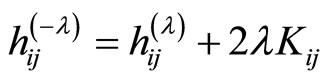
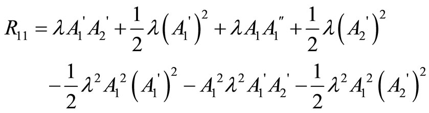
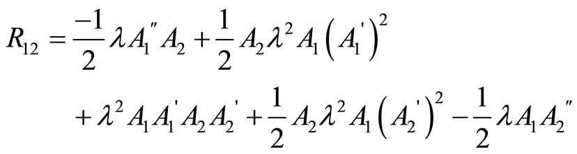
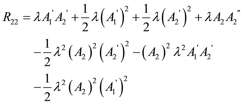
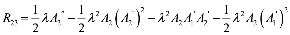
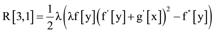
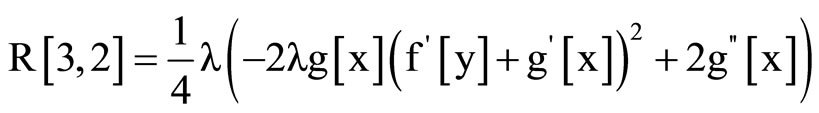
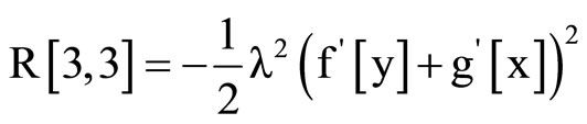
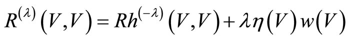
If  are the components of the Ricci tensor with respect to the metric given in (20), then
 (23)
(23)
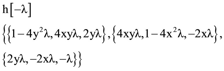
where  is obtained by flipping the sign in(20)
And R is the Ricci scalar
Proof
We will just replace the coefficients of  and
and  in the relation (24), and next we will use the following relation to compare the two results :
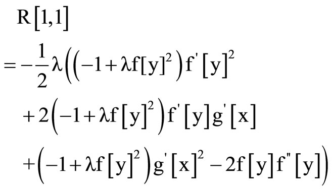
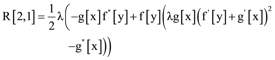
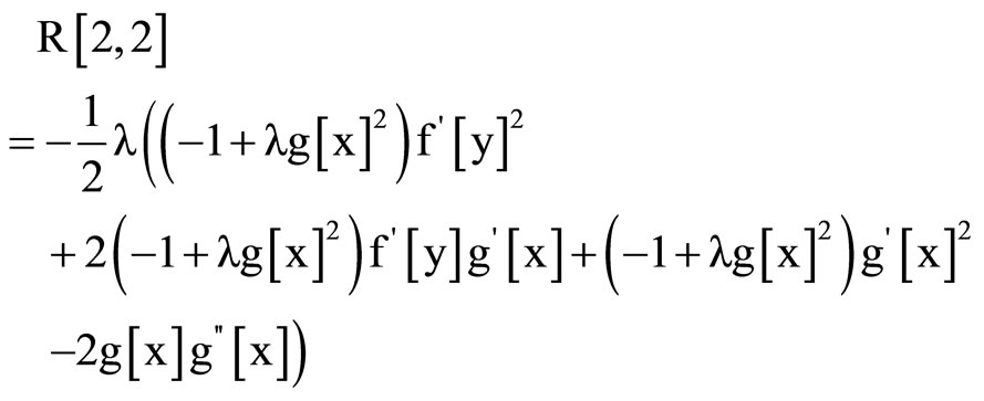
For this, we use the mathematica program.
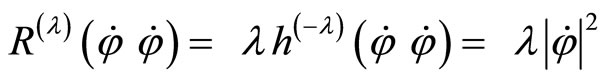
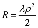
1) We have , then

And the Ricci scalar is :
 (24)
(24)
2) we put :
 ,
, 
Clear [coord, metric, inversemetric, affine, riemann, ricci, scalar, x, y, t, A, B]


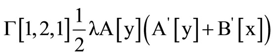
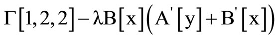
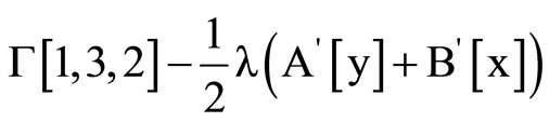

 ,
,

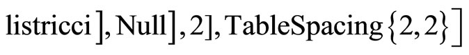

Remarque:
To show the values of the Riemann tensor ,add the following command :

Lemma 3
Consider the curve
 (25)
(25)
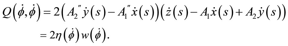
Then
Proof
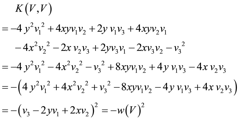
Let 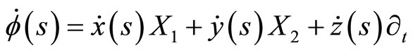 be the tangent vector field Then
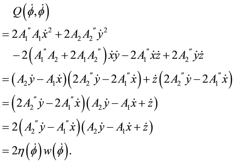
We note that  and w measure the departure from the Heisenberg structure and horizontality respectively. When the structure is Heisenberg,
  and when V is horizontal,
 .
.
In the following we give a global interpretation for the difference  in terms of the horizontal distribution
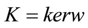 .
.
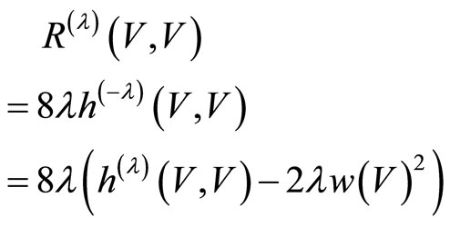
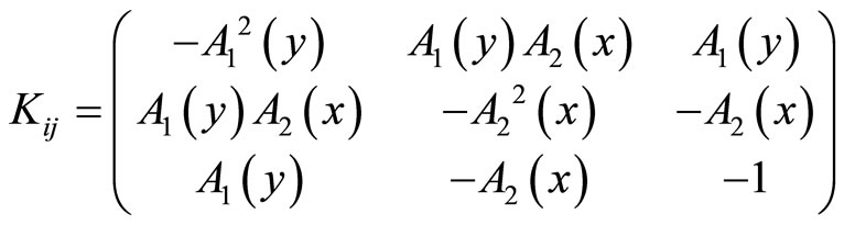
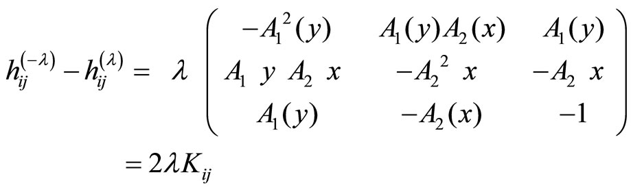
Lemma 4
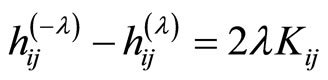 (26)
(26)
With
Furthermore
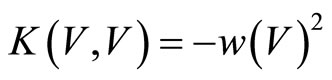
Proof
For the relation (2.28):
For the second part we have:
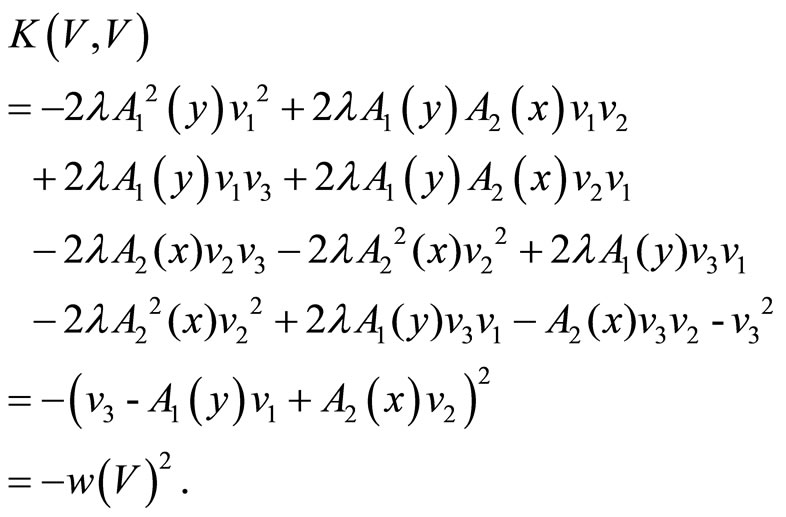
Denote ,
, 
Denote also
 .
.
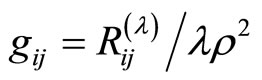
Theorem 2
 and
and 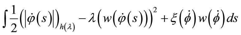 reach the extrema for the same functions. In particular, the extrema will be geodesics in the metric
  and obey the equation
  where
where  is the Levi-Civita type connection defined by
Proof
From Lemma 2 and Lemma 3 we have
Using Lemma 4 we get

From (24)
Hence
The last equation can be written also as
which completes the proof.
4. Natural Levi-Civita Connection on Heisenberg Group [6]
We start with the properties of the Levi-Civita connection on . For each metric
  one has a natural Levi-Civita connection
  defined by
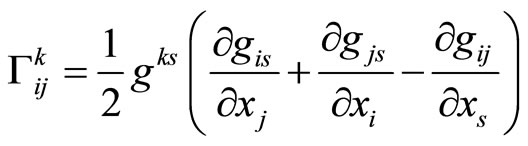
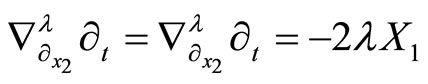
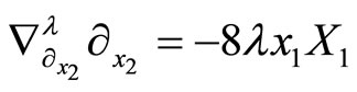
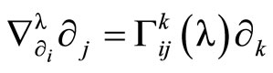 (27)
(27)
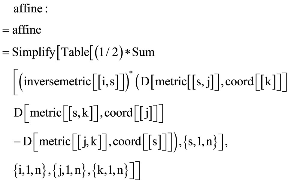
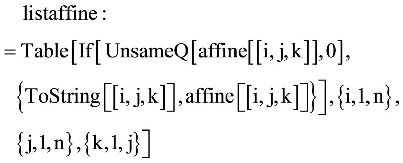
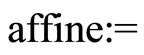
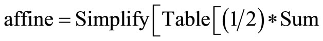
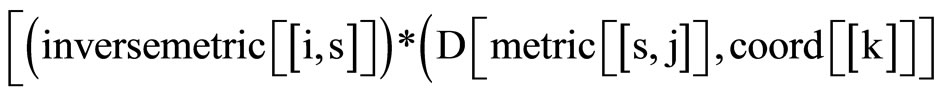
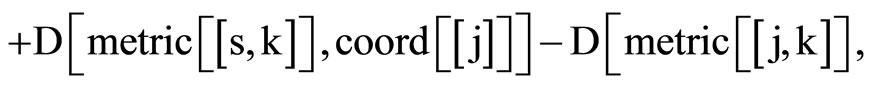
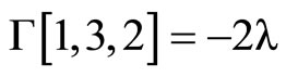
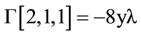
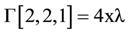
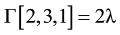
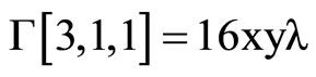
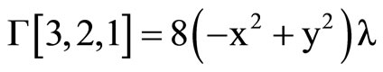
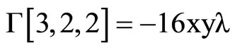
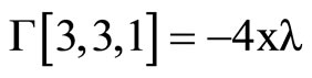
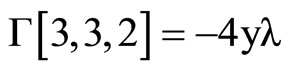
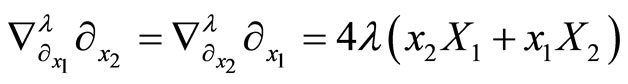
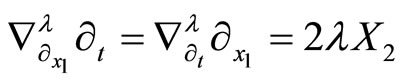
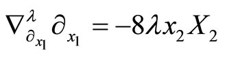
where the Christoffel symbols are defined by the metric (1).They depend linearly on  and are given by using Mathematica program.


The following result states tha the Levi-Civita connection with respect to ,
,  ,
,  is always a linear combination of
  and
and  and hence belongs to the distribution generated by this vectors
Lemma 5
For every  we have
 ,
,

Proof
For the demonstration, see in [6]
The following proposition shows that the vector fields are geodesic vector fields.
Proposition 2
For every 
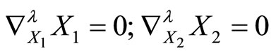
Proof
See in [6]
5. Conclusions
In this paper, we have proposed an approach for the implementation of the Geodesic method with constraints on Heisenberg Manifolds by including more details with complete proofs that are required for the implementation.
The method has been implemented on Mathematic.8. This implementation extends the rang of applications of the method with more flexibility and rapidity. It has been shown that the Ricci tensor can easily be determined using our implementation.
REFERENCES
- O. Calin and V. Mangione, “Geodesics with Constraints on Heisenberg Manifolds,” Results in Mathematics, 2003, pp. 44-53. http://people.emich.edu/ocalin/Papers_research/4.pdf
- M. Bonnefont, “Functional Inequality for Heat Kernels Sub-Elliptical,” Ph.D. Thesis, Paul Sabatier University, Toulouse, 2009.
- D.-C. Chang, I. Markina and A. Vasil’ev, “Sub-Riemannian Geodesics on the 3-D Sphere,”2008. http://arxiv.org/pdf/0804.1695.pdf
- L. Capogna, D. Danielli, S. Pauls and J. Tyson, “An Introduction to the Heisenberg Group and the Sub-Riemannian Isoperimetric Problem,” Die Deutsche Bibliothek, Deutsche Nationalbibliografie, 2007.
- R. Beals, B. Gaveau and P. C. Greiner, “Hamilton-Jacobi Theory and the Heat Kernel on Heisenberg Groups,” journal of mathéMatiques Pures et Appliquées, Vol. 79, No. 7, 2000, pp. 633-689. doi:10.1016/S0021-7824(00)00169-0
- O. Calin, “The Missing Direction and Differential Geometry on Heisenberg Manifolds,” Ph.D. Thesis, Toronto University, Toronto, 2000.