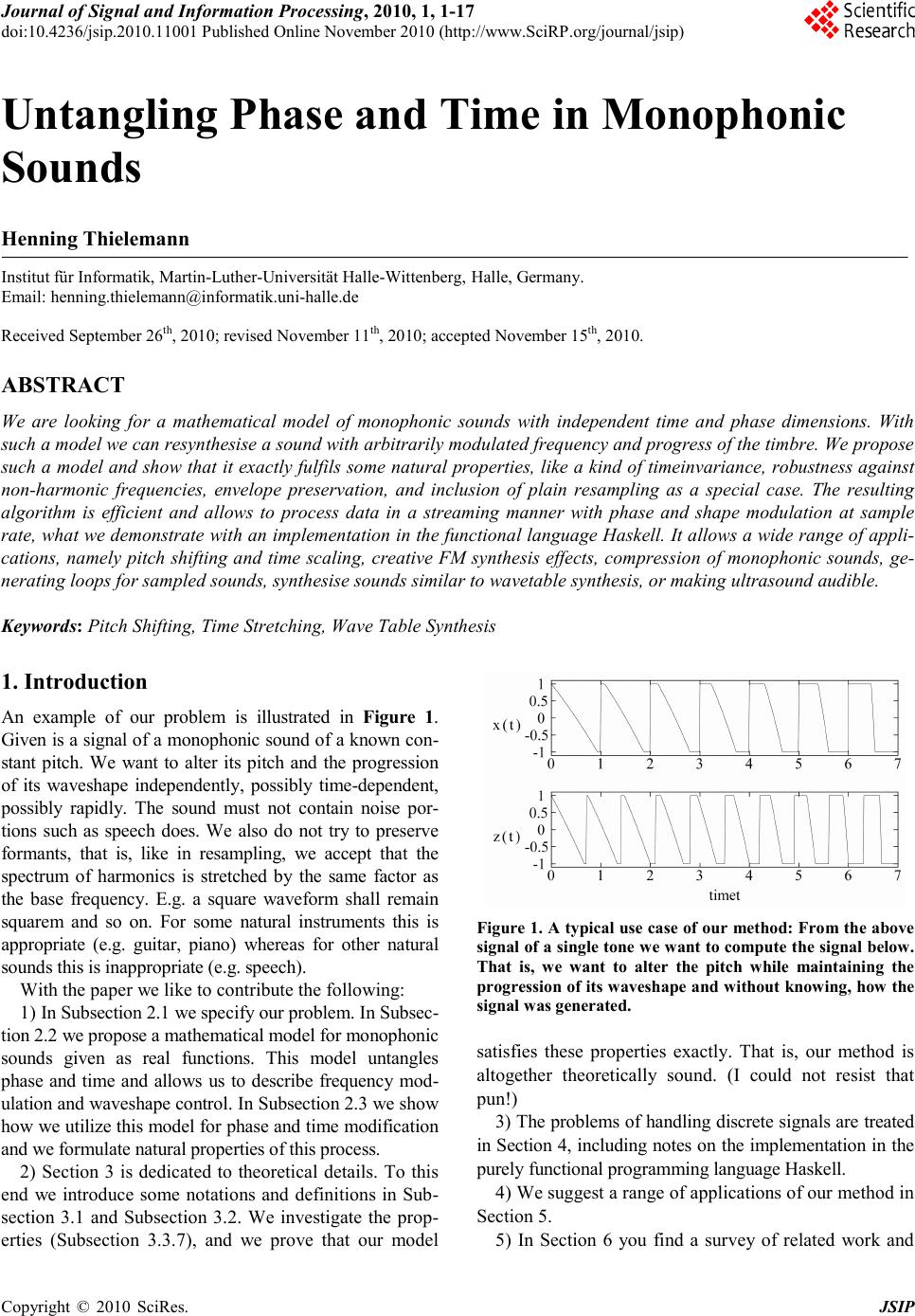Journal of Signal and Information Processing, 2010, 1, 1-17
doi:10.4236/jsip.2010.11001 Published Online November 2010 (http://www.SciRP.org/journal/jsip)
1
Untangling Phase and Time in Monophonic
Sounds
Henning Thielemann
Institut für Informatik, Martin-Luther-Universität Halle-Wittenberg, Halle, Germany.
Received September 26th, 2010; revised November 11th, 2010; accepted November 15th, 2010.
ABSTRACT
We are looking for a mathematical model of monophonic sounds with independent time and phase dimensions. With
such a model we can resynthesise a sound with arbitrarily modulated frequency and progress of the timbre. We propose
such a model and show that it exactly fulfils some natural properties, like a kind of timeinvariance, robustness against
non-harmonic frequencies, envelope preservation, and inclusion of plain resampling as a special case. The resulting
algorithm is efficient and allows to process data in a streaming manner with phase and shape modulation at sample
rate, what we demonstrate with an implementation in the functional language Haskell. It allows a wide range of appli-
cations, namely pitch shifting and time scaling, creative FM synthesis effects, compression of monophonic sounds, ge-
nerating loops for sampled sounds, synthesise sounds similar to wavetable synthesis, or making ultrasound audible.
Keyword s: Pitch Shifting, Time Stretching, Wave Table Synthesis
1. Introduction
An example of our problem is illustrated in Figure 1.
Given is a signal of a monophonic sound of a known con-
stant pitch. We want to alter its pitch and the progression
of its waveshape independently, possibly time-dependent,
possibly rapidly. The sound must not contain noise por-
tions such as speech does. We also do not try to preserve
formants, that is, like in resampling, we accept that the
spectrum of harmonics is stretched by the same factor as
the base frequency. E.g. a square waveform shall remain
squarem and so on. For some natural instruments this is
appropriate (e.g. guitar, piano) whereas for other natural
sounds this is inappropriate (e.g. speech).
With the paper we like to contribute the following:
1) In Subs ection 2.1 we specify our problem. In Subsec-
tion 2.2 we propose a mathematical model for monophonic
sounds given as real functions. This model untangles
phase and time and allows us to describe frequency mod-
ulation and waveshape control. In Subsection 2.3 we show
how we utilize this model for phase and time modification
and we formulate natural properties of this process.
2) Section 3 is dedicated to theoretical details. To this
end we introduce some notations and definitions in Sub-
section 3.1 and Subsectio n 3.2. We investigate the prop-
erties (Subsectio n 3.3.7), and we prove that our model
Figure 1. A typical use case of our method: From the above
signal of a single tone we want to compute the signal below.
That is, we want to alter the pitch while maintaining the
progression of its waveshape and without knowing, how the
signal was generated.
satisfies these properties exactly. That is, our method is
altogether theoretically sound. (I could not resist that
pun!)
3) The problems of handling discrete signals are treated
in Section 4, including notes on the implementation in the
purely functional programming language Haskell.
4) We suggest a range of applications of our method in
Section 5.
5) In Section 6 you find a survey of related work and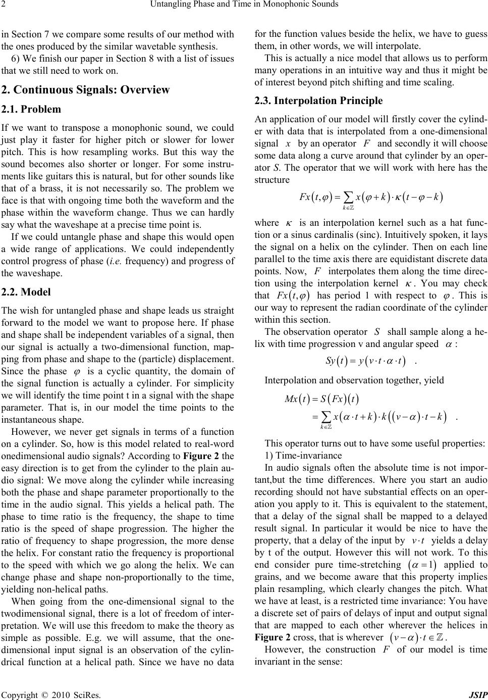

Untangling Phase and Time in Monophonic Sounds
2
in Section 7 we compare some results of our method with
the ones produced by the similar wavetable synthesis.
6) We finish our paper in Section 8 with a list of issues
that we still need to work on.
2. Continuous Signals: Overview
2.1. Problem
If we want to transpose a monophonic sound, we could
just play it faster for higher pitch or slower for lower
pitch. This is how resampling works. But this way the
sound becomes also shorter or longer. For some instru-
ments like guitars this is natural, but for other sounds like
that of a brass, it is not necessarily so. The problem we
face is that with ongoing time both the waveform and the
phase within the waveform change. Thus we can hardly
say what the waveshape at a precise time point is.
If we could untangle phase and shape this would open
a wide range of applications. We could independently
control progress of phase (i.e. frequency) and progress of
the waveshape.
2.2. Model
The wish for untangled phase and shape leads us straight
forward to the model we want to propose here. If phase
and shape shall be independent variables of a signal, then
our signal is actually a two-dimensional function, map-
ping from phase and shape to the (particle) displacement.
Since the phase
ϕ
is a cyclic quantity, the domain of
the signal function is actually a cylinder. For simplicity
we will identify the time point t in a signal with the shape
parameter. That is, in our model the time points to the
insta nt a ne o u s s hape.
However, we never get signals in terms of a function
on a cylinder. So, how is this model related to real-word
oned imensional audio signals? According to Figure 2 the
easy direction is to get from the cylinder to the plain au-
dio signal: We move along the cylinder while increasing
both the phase and shape parameter proportionally to the
time in the audio signal. This yields a helical path. The
phase to time ratio is the frequency, the shape to time
ratio is the speed of shape progression. The higher the
ratio of frequency to shape progression, the more dense
the helix. For constant ratio the frequency is proportional
to the speed with which we go along the helix. We can
change phase and shape non-proportionally to the time,
yielding non-helical paths.
When going from the one-dimensional signal to the
twodimensional signal, there is a lot of freedom of inter-
pretation. We will use this freedom to make the theory as
simple as possible. E.g. we will assume, that the one-
dimensional input signal is an observation of the cylin-
drical function at a helical path. Since we have no data
for the function values beside the helix, we have to guess
them, in other words, we will interpolate.
This is actually a nice model that allows us to perform
many operations in an intuitive way and thus it might be
of interest beyon d pitch shifting and time scaling.
2.3. Interpolation Principle
An application of our model will firstly cover the cylind-
er with data that is interpolated from a one-dimensional
signal
x
by an operator
F
and secondly it will choose
some data along a curve around that cylinder by an oper-
ator S. The operator that we will work with here has the
structure
()() ()
,
k
Fx txktk ϕϕ κϕ
∈
=+ ⋅−−
∑

where
κ
is an interpolation kernel such as a hat func-
tion or a sinus cardinalis (sinc). Intuitively spoken, it lays
the signal on a helix on the cylinder. Then on each line
parallel to the time axis there are equidistant discrete data
points. Now,
F
interpolates them along the time direc-
tion using the interpolation kernel
κ
. You may check
that
( )
,Fx t ϕ
has period 1 with respect to
ϕ
. This is
our way to represent the radian coordinate of the cylinder
within this section.
The observation operator
S
shall sample along a he-
lix with time progression v and angular speed
α
:
( )()
.Sy tyv tt α
=⋅⋅ ⋅
Interpolation and observation together, yield
( )()( )
() ()
( )
.
k
Mx tSFxt
x tkkvtk
αα
∈
=
=⋅+ ⋅−⋅−
∑

This operator turns out to have some useful properties:
1) Time-i nva r iance
In audio signals often the absolute time is not i mpor-
tant,but the time differences. Where you start an audio
recording should not have substantial effects on an oper-
ation you apply to it. This is equivalent to the statement,
that a delay of the signal shall be mapped to a delayed
result signal. In particular it would be nice to have the
property, that a delay of the input by
vt⋅
yields a delay
by t of the output. However this will not work. To this
end consider pure time-stretchin g
( )
1 α =
applied to
grains, and we become aware that this property implies
plain resampling, which clearly changes the pitch. What
we have at least, is a restricted time invariance: You have
a discrete set of pairs of delays of input and output signal
that are mapped to each other wherever the helices in
Figure 2 cross, that is wherever
( )
vt α − ⋅∈
.
However, the construction
F
of our model is time
invari a nt in the sense: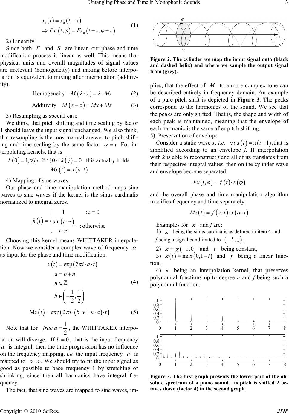

Untangling Phase and Time in Monophonic Sounds
3
( )()
( )()
10
10
,,
xtxt x
Fx tFxt ϕτϕ τ
= −
⇒= −−
(1)
2) Linearity
Since both
F
and
S
are linear, our phase and time
modification process is linear as well. This means that
physical units and overall magnitudes of signal values
are irrelevant (homogeneity) and mixing before interpo-
lation is equivalent to mixing after interpolation (additiv-
ity).
( )
Homogeneity M xMx λλ ⋅=⋅
(2)
( )
AdditivityM xzMxMz+=+ (3)
3) Resampling as special case
We think, that pitch shifting and time scaling by factor
1 should leave the input signal unchanged. We also think,
that resampling is the most natural answer to pitch shift-
ing and time scaling by the same factor
v α =
For in-
terpolating kernels, that is
(){ }()
01,\ 0 :0k jkj= ∀∈= this actually holds.
( )()
Mx txv t= ⋅
4) Mapping of sine waves
Our phase and time manipulation method maps sine
wav es to sine waves if the kernel is the sinus cardinalis
normalized to integral zeros.
( )( )
1 :0
sin : otherwise
t
kt t
t
π
π
=


=⋅

⋅

Choosing this kernel means WHITTAKER interpola-
tion. Now we consider a complex wave of frequency
α
as input for the phase and time modification.
( )()
exp 2
11
,
22
xt iat
a bn
n
b
π = ⋅⋅
= +
∈

∈−



(4)
( )()
( )
Mexp 2xtibv + nat π =⋅⋅⋅⋅
(5)
Note that for
1
2
frac a =
, the WHITTAKER interpo-
lation will diverge.
If 0b=
, that is the input frequency
a
is integral, then the time progression has no influence
on the frequency mapping, i.e. the input freq uenc y
a
is
mapped to
a α ⋅
. We should try to fit the input signal as
good as possible to base frequency 1 by stretching or
shri nk in g, since then all harmonics have integral fre-
quency.
The fact, that sine waves are mapped to sine waves, im-
Figure 2. The cylinder we map the input signal onto (black
and dashed helix) and where we sample the output signal
from (grey).
plies, that the effect of
M
to a more complex tone can
be described entirely in frequency domain. An example
of a pure pitch shift is depicted in Figure 3. The peaks
correspond to the harmonics of the sound. We see that
the peaks are only shifted. That is, the shape and width of
each peak is maintained, meaning that the envelope of
each harmonic is the same after pitch shifting.
5). Preservation of envelope
Consider a static wave x, i. e.
( )()
1txt xt∀=+
,that is
amplified according to an envelope f. If interpolation
with k is able to reconstruct f and all of its translates from
their respective integral values, then on the cylinder wave
and envelope become separated
()( )()
,Fx tftx ϕϕ = ⋅
and the overall phase and time manipulation algorithm
modifies frequency and time separately:
( )()()
Mx tfv txt
α =⋅⋅ ⋅
Examples for
κ
and f are:
1)
κ
being the sinus cardinalis as defined in item 4 and
f being a signal bandlimited to
( )
11
22
,−
,
2)
(
]
= 1,0
κχ −
and
f
being constant,
3)
( )()
= max0,1tt κ −
and
f
being a linear func-
tion,
4)
κ
being an interpolation kernel, that preserves
pol ynomial func tions up to degree n and f being such a
polynomial function.
Figure 3. The first graph presents the lower part of the ab-
solute spectrum of a piano sound. Its pitch is shifted 2 oc-
taves down (factor 4) in the second graph.

Untangling Phase and Time in Monophonic Sounds
4
3)
κ
being an interpolation kernel, that preserves
polynomial functions up to degree
n
and
f
being
such a polynomial function.
3. Continuous Signals: Theory
In this section we want to give proofs of the statements
found in Section 2 and we want to check what we could
have done alternatively given the properties that we
found to be useful. You can safely skip the entire section
if you are only interested in practical results and applica-
tions.
3.1. Notation
In order to give precise, concise, even intuitive proofs,
we want to introduce some notations.
In signal processing literature we find often a term like
( )
xt
being called a signal, although from the context
you derive, that actually x is the signal and thus
( )
xt
denotes a displacement value of that signal at time t. We
like to be more strict in our paper. We like to talk about
signals as objects without always going down to the level
of single signal values. Our notation should reflect this
and should clearly differentiate between signals and sig-
nal values. This way, we can e.g. express a statement like
“delay and convolution commute” by
()( )
=t xyxty∗∗
(cf. (22)) which would be more difficult in a pointwise
and correct (!) notation.
This notation is inspired by functional programming,
whe re functions that process functions are called high-
er-order functions. It allows us to translate the theory
described here almost literally to functional programs
and theorem prover modules. Actually some of the theo-
rems stated in this paper have been verified using PVS
[1]. For a more detailed discussion of the notation, see
[2].
In our notation function application has always higher
precedence than infix operators. Thus
Qx t→
means
( )
Qx t→
and not
( )
Qx t→
. Function application is
left associative, that is,
( )
Qx t
means
()( )
Qx t
and not
( )
( )
Qxt
. This is also the convention in Functional
Analysis. We use anonymous functions, also known as
lambda expressions. The expression
xY
denotes a
function
f
where
( )
=xf xY∀
and
Y
is an ex-
pression that usually contains
x
. Arithmetic infix op er-
ators like “
+
” and “
⋅
” shall have higher precedence than
the mapping arrow, and logical infix operators like “
=
”
and “
∧
” shall have lower precedence. That is,
( )
=tf tf ττ −
means
( )()
( ) ( )
( )
( )
=tf tgtfg τ ττ
−+ −+
.
1) Definitio n (Function set). With
AB→
we like to denote the set of all functions mapping from
set
A
to set
B
. This operation is treated right associa-
tive, that is,
ABC→→
means
()A BC
→→, not
()ABC→→
. This convention matches the convention
of left associative function application.
3.2. Basic functions
For the description of the cylinder we first need the no-
tion of a cyclic quantity.
2) Definition (Cyclic quantity). Intuitively spoken,
cyclic (or periodic) quantities are values in the range
[
)
0,1
that wrap around at the boundaries. More precisely,
a cyclic quantity
ϕ
is a set of real numbers that all have
the same fractional part. Put differently, a periodic quan-
tity is an equivalence class with respect to the relation,
that two numbers are considered equivalent when their
diffe r enc e is integral. In terms of a quotient space this
can concisely be written as
. ϕ ∈

3) Definition (Periodisation). Periodisation c means
mapping a real value to a cyclic quantity, i.e. choosing
the equivalence class belonging to a representative.
( )
{ }
:
c
pcp p
qqp
∈→
∀∈=+
= −∈




It holds
( )
0c=
. We define the inverse of
c
as
picking a representative from the range
[
)
0;1
.
( ) [ )
1
1
0,1
c
c ϕ ϕϕ
−
−
∈→
∀∈ ∈∩




In a computer program, we do not encode the elements
of


by sets of numbers, but instead we store a rep-
resentative between 0 and 1, including 0 and excluding 1.
Then c is just the function, that computes the fractional part,
i.e.
c t = tfloor t.−
A function y on the cylinder is thus from
( )
V×→


, where
V
denotes a vector space. E.g. for
V=
we have a mono
signal, for
V= ×
we obtain a stereo signal and so on.
The conversion
S
from the cylinder to an audio sig-
nal is entirely determined by given phase control curve g
and shape control curve h. It consists of picking the val-
ues from the cylinder along the path that corresponds to
these control curves.

Untangling Phase and Time in Monophonic Sounds
5
( )
( )
( )
,hg
S VV∈ ×→→→



(6)
( )( )( )
( )
,
,
hg
Sytyht gt∈
(7)
For the conversion F from a prototype audio signal to
a cylindrical model we have a lot of freedom. In Section
2.3 we ave seen what properties a certain F has, that we
use in our implementation. we will going on to check
what choices for F wehave, given that these properties
hold. For now we will just record, tha t
( )
( )
( )
FV V∈→→ ×→



3.3. Properties
3.3.1. Time-Invariance
4) Def inition (Translation, Rotation). Shifting a signal x
forward or backward in time or rotating a waveform with
respect to its phase shall be expressed by an intuitive
arrow notation that is inspired by [3,4] and was already
successfully applied in [2]:
()( )()
xt xt ττ →=−
(8)
()( )()
xt xt ττ →=+
(9)
For a cylindrical function we have two directions, one
for rotation and one for translation. We define analo-
gous l y
( )
( )
( )()
,, ,yt yt ταϕτϕ α → =−−
(10)
( )
( )
( )()
,, ,ytyt ταϕτϕ α → =++
(11)
The first notion of time-invariance that comes to mind,
can be easily expressed using the arrow notation by
()( )
( )
,0t FxtFxtc∀→= →
. However, this will not
yield any useful conversion. Shifting the time always
includes shifting the phase and our notion of
time-invariance must respect that. We have already given
an according definition in (1) that we can now write us-
ing the arrow notation.
5) Definition (Time-invariant cylinder interpolation).
We call an interpolation operator F time-invariant when-
ever it satisfies
()( )
( )
,xtFxtFxtct∀∀→ =→ (12)
Using this definition, we do not only force F to map
translations to translations, but we also fix the factor of
the translation distance to 1. That is, when shifting an
input signal x, the according model Fx is shifted along
the unit helix, that turns once per time difference 1.
Enforcing the time-invariance property restricts our
choice of F considerably.
( )
( )
( ) ( )
( )
( )
()( )
( )
,
, 0,
0,
Fx t
Fx tctct
F xtct
ϕ
ϕ
ϕ
=←−
=←−
We see, that actually only a ring slice of
( )
Fx t←
time point zero is required and we can substitute
( )()
0,Ix Fx ϕϕ =
I is an operator from
( )
( )
VV→→ →


, that turns a straight signal into
a waveform. Now we know, that time-invariant interpo-
lations can only be of the form
()()( )
( )
,FxtI xtct ϕϕ =→−
(13)
or more concisely
()()( )
,FxtI xtct ϕϕ = →→
(14)
The last line can be read as: In order to obtain a ring
slice of the cylin drical model at time t, we have to move
the signal, such that time point t becomes point 0, then
apply I to get a waveform on a ring, then rotate back that
ring correspondingly.
We may check, that any F defined this way is indeed
timeinvariant in the sense of (12).
()( )
( ) ( ) ( )
( ) ( ) ( ) ( )
( ) ( ) ()() ( ) ( )
( ) ( )
( ) ( )
( )
( )
,
,
,,
Fx xt
Ix tc
Ixtc
I xttctct
Fxtc t
Fxt ct
τϕ
τϕ τ
τ ϕτ
τ τττ
τϕ
τϕ
→
=→← −
= ←−−
=←−−−− −
= −−
= →
3.3.2. Linearity
We like that our phase and time modification process is
linear (as in (2) and (3)). Since sampling S from the cy-
linder is linear, the interpolation F to the cylinder must
be linear as well.
( )
( )
Homogeneity
Additivity
F xFx
F xzFxFz
λλ ⋅=⋅
+= +
The properties of F are equivalent to
( )
( )
I xIx
I xzIxIz
λλ
⋅=⋅
+=+
3.3.3. Static wave preservation
Another natural property is, that an input signal consist-
ing of a wave of constant shape is mapped to the cylinder
where each ring contains that waveform. A static wave-
form can be written concisely as
wc
. It denotes the
function composition of
w
and
c
, that is,
w
is applied

Untangling Phase and Time in Monophonic Sounds
6
to the result of
c
, for example
()( )( )
( )
2.3 =0.3w cwc
.
Thus
w
and
wc
both represent periodic functions,
but
w
has domain


and thus is periodic by its
type, whereas
wc
is an ordinary real function, that
happens to satisfy the periodicity property
()=1()
wc wc

. We can write our requirement as
()()( )
,= .tFwc tw φ ϕϕ ∀∀ 
As an example we have a constant interpolation
( )
()( )
( )
( )
1
1
,
Ix xc
Fxtxt cct ϕϕ
−
−
=
=+−

We illustrate the constant interpolation in Figure 4,
but with a sine wave, that does not have frequency 1, and
thus looks for the interppoow it preserves static waves.
We can consider an input signal of the form
wc
as
a wave with constant envelope and we will generalise
this to other envelopes in Sub s ection 3.3.6.
3.3.4. Mapping of Pure Sine Waves
We like to derive, how frequencies are mapped when
converting from an audio signal to the cylindrical model
and observing the signal along a different but uniform
helix. To this end, we need an interpolation that maps
sine waves to sine waves. Actually, the Whittaker inter-
polation has this property.
( )
( )
sin
sin 1lim
1 :0
sin : otherwise
t
ct
t
t
t
τ
τπ
τπ
π
π
→
⋅
=⋅
=


=⋅

⋅

Figure 4. Constant interpolation (below) of a sine wave
(above) that is out of sync. The interpolation picture repre-
sents the surface
( )
,1yt ϕ = −
and a white dot repre- sents
1. The sine wave can be found in the interpolation image at
the right border of each of the skew stripes. Along the ver-
tical line from bottom to top you find the first period of the
input signal, where “first” is measured from time point 0.
()( )()
,sin 1Fx txct
τϕ
ϕτ τ
∈
= ⋅−
∑
(15)
Since ϕ ∈

, when
τϕ ∈
then
τ
assumes all
values that differ from
( )
1
c ϕ
− by an integer. The infi-
nite sum
( )
f
τϕ
τ
∈
∑
shall be understood as
[ ]
( )
,
lim
nnn
f
τϕ
τ
→∞ ∈−
∑
.
The proof of
F
being time-invariant according to
time-invariance is deferred to kernel-interpola tion-time -
invariant, where we perform the proof for any interpo-
lating kernel, not just
1sinc
.
We will now demonstrate, that
1sinc
-interpolation
preserves sine waves and how frequencies are mapped.
Mapping a complex sine wave to the cylinder Since
exponential laws are much easier to cope with than addi-
tion theorems for sine and cosine, we use a complex
wave defined by
( )
1= exp2.cis tit
π
⋅
For the following derivation we need the Whittaker-
Shannon interpolation formula [5] in the form
()
11
,
22
b∀∈−
()( )()( )
( )
11 =11
1
k
cis bksinc tkcis btsine tk
cisbt
∈
⋅ ⋅−⋅⋅−
= ⋅
∑

(16)
We choose a complex wave of frequency
a
as input
for the conversion to the cylinder. The fractional fre-
quency part b and the integral frequency
n
are cho-
sen as in decompose-freque ncy
n
are chosen as in (4)
( )()
( )
11
22
1
,
x tcisat
with abn
n
b
= ⋅
= +
∈
∈−

This choice implies the following interpolation result
( )()()
( )()()()
( )()()
( )()
( )
( )
()( )
( )
1
,1sin 1
,11sin1
because
11sin1
11
1
,1
k
k
Fx tcisact
Fxtcis acis aktk
ab
cisacisb ktk
cis acis bt
cisbtn
Fx tcisb tnc
τ
ϕ ττ
τϕ
ϕτ τ
ττ
ττ
τ
ϕϕ
∈
∈
∈
−
=⋅⋅ −
∀∈
=⋅ ⋅⋅⋅−−
−∈
=⋅ ⋅⋅ ⋅−−
=⋅⋅⋅−
=⋅+ ⋅
=⋅+ ⋅
∑
∑
∑




(17)
The result can be viewed in Figure 5. We obtain, that
for every t the function on a ring slice
( )
,Fx t ϕϕ 
is a

Untangling Phase and Time in Monophonic Sounds
7
Figure 5. The sine wave as in Figure 4 is interpolated by
WHITTAKER interpolation. Along the diagonal lines you
find the original sine wave.
sine wave with the integral frequency n that is closest to
a. That is, the closer a is to an integer, the more harmon-
ics of a non-sine wave are mapped to corresponding
harmonics in a ring slice of
Fx
.
Mapping a complex wave from the cylinder to an
audio signal For time progression speed v and frequency
α
we get
( )() ( )
( )
( ) ( )
( )
( )
( )
( )
1
1
,
1
because
1
1
ztFxvt cat
cis bvtnccat
cc
cis bvtnat
cisbvnat
τ ττ
−
−
=⋅⋅
=⋅⋅+⋅⋅
∀∈ −∈
=⋅⋅+ ⋅ ⋅
=⋅+⋅ ⋅

This proves (5).
3.3.5. Interpolation using kernels
Actually, for the two-dimensional interpolation F we can
use any interpolation kernel
κ
, not only sinc1 as in (15).
()( )()
,Fx txt
τϕ
ϕτκ τ
∈
= ⋅−
∑
(18)
The constant interpolation corresponds to
( ]
1,0
κχ
−
=
Linear interpolation is achieved using a hat function. 6
Lemma (Time invariance of kernel interpolation). The
operator F defined with an interpolation kernel as in (18)
is time-invariant according to Definition 5.
Proof.
( )()( )()()
( )()( )
( )
( )
( )
( )
( )
( )
( ) ( )
( )
,
,,
cd
Fxdtxd t
x dtdd
x td
Fxdcdt
τϕ
τϕ
τϕ
ϕτκ τ
τκ τ
τκ τ
ϕ
∈
∈
∈−
→= →⋅−
=−⋅ −−−
=⋅−−
= →
∑
∑
∑
Conversely, we like to note, that kernel interpolation is
not the most general form when we only require time-
invariance, linearity and static wave preservation.
The following considerations are simplified by rewrit-
ing general kernel interpolation to a more functional style
using a discretisation operator and a mixed discrete/con-
tinuous convolution.
7) Definition (Quantisation). With quantisation we
mean the operation that picks the signal values at integral
time points from a continuous signal.
() ()
( )()
QV V
nQxn xn
∈→→→
∀∈ =


(19)
Here is, how quantisation operates on pointwise mul-
tiplied signals and on periodic signals:
( )
QxzQx Qz⋅= ⋅
(20)
()( )()
( )
0nQw cnwc∀∈ =
(21)
8) Definition (Mixed Convolution). For
uV∈→
and
x∈→
then mixed discrete/continuous convo-
lution is defined by
()()()()
k
u x tukxtk
∈
∗ =⋅−
∑

We can express mixed convolution also by purely dis-
crete convolutions:
( )
( )
( )
Qu xtuQxt∗←=∗ ←
It holds
( )()
uxt uxt∗→=∗→
(22)
because translation can be written as convolution with a
translated DIRAC impulse and convolution is associative
in this case (and generally when infinity does not cause
problems). Thus we will omit the parentheses. We like to
note, that this example demonstrates the usefulness of the
functional notation, since without it even a simple state-
ment like (22) is hard to formulate in a correct and un-
ambiguous way.
These notions allow us to rewrite kernel interpolation
(18):
()()()
( )
( )()
,
,
k
Fx tx ktk
tFx tQx
τϕ ϕτκτ
τϕϕτ κτ
∈
∀∈=+⋅−+
∀∈=←∗→
∑


(23)
The last line can be read as follows: The signal on the
cylin der along a line parallel to the time axis can be ob-
tained by taking discrete points of x and interpolate them
using the kernel
κ
.
3.3.6. Envelope preservation
We can now generalise the preservation of static waves
from Subsec tio n 3.3.3 to envelopes different from a con-
stant function.
9) Lemma. Given an envelope f from
→
and an
interpolatio n kernel
κ
that preserves any translated
version of f, i.e.

Untangling Phase and Time in Monophonic Sounds
8
( )
,tQft ft
κ ∀←∗= ←
(24)
then and only then, a wave of constant shape w enve-
loped by f is converted to constant waveshapes on the
cylinder rings enveloped by f in time direction:
( )
( )
()( )()
,F fwctftw ϕϕ ⋅=⋅
(25)
Proof.
( ) ( ) ( )
( )
( ) ( )
()() ( )
( )
( )()
,tFfwct
Q f wc
Qfw c
w Qf
τϕ ϕ
τκτ
τϕ κτ
ϕτκ τ
∀∈ ⋅
=⋅← ∗→
=← ⋅←∗→
=⋅← ∗→



Now the implication (24)
⇒
(25) should be obvious,
whereas the conve r se (25)
⇒
(24) can be verified by
setting
( )
1w ϕϕ ∀=
.This special case means that the
envelope f used as input signal is preserved in the sense
()( )
,Fftft ϕ =
10) Corollary When we convert back to a
one-dimensional audio signal under the condition (24),
then the time control only affects the envelope and the
phase control only affects the pitch:
( )
( )
( )
()()
,hg
SFfwcf hwg⋅=⋅ 
3.3.7. Special Cases
As stated in item 3 of Section 2.3 we like to have resam-
pling as special case of our phase and time manipulation
algorithm. It turns out, that this property is equivalent to
putting the input signal x on the diagonal lines as in Fig-
ure 4 and Figure 5. We will derive, what this imposes on
the choice of the kernel
κ
when F is defined via a ker-
nel as in (23).
11) Lemma. For F defined by
( )()
,tFx tQx τϕϕτ κτ ∀∈=←∗ →
it holds
()( )
( )
,xtxtFxtct∀∀∈ =
(26)
if and only if
,Q κδ =
that is,
κ
is a so called interpolating kernel.
Here,
δ
is the discrete DIRAC impulse, that is
( )
1 :0
0:
k
kkotherwise δ
=

∀∈ =



Proof. “
⇒
”
( )( ) ( )
( ) ( ) ()
,x txtFxtct
Qx ttt κ
∀∀∈ =
= ←∗→

consider only
t∈
and rename it to k
( )()
( )
( )
()( )
( )
( )
x kxkQxkkk
Qx k
xQxQ Qx
QxQdiscrete convolution
κ
κ
κ
κ
∀∀ ∈=←∗→
= ∗
∀=∗
= ∗

“
⇐
”
Conver sely, every interpolating kernel _ asserts (26):
( )() ( ) ( )
()()
( ) ( )
( )
( ) ( ) ( )
( ) ( ) ( )
()( )
( )
0
0
0
0
0
x kxkQxkkk
Qx t
QQx t
Qxt Q
Qx t
xt
xt
κ
κ
κ
κ
δ
∀∀ ∈=→∗→
= ←∗
= ←∗
= ←∗
= ←∗
= ←
=

Now, when our conversion from the cylinder to the
oned imensional signal does only walk along the unit he-
lix, we get general time warping as special case of our
method:
()( )()
( )
( )
( )
( )
,
,
hc h
SFxtFxh tc h t
t xht
xh
=
=
=




For
idh=
we get the identity mapping, for
( )
ht vt=⋅ we get resampling by speed factor v.
4. Discrete Signals
For the application of our method to sampled signals we
could interpolate a discrete signal u containing a wave
with period T, thus getting a continuous signal x with
( )
( )
n
T
x un=
and proceed with the technique for con-
tinuous signals from Section 2. However, when working
out the interpolation this yields a skew grid with two al-
ternating cell heights and a doubled number of parallelo-
gra m cells, which seems to be unnatural to us. Additional-
ly it would require three distinct interpolations, e.g. two
distinct interpolations in the unit helix direction and one
interpolation in time direction. Instead we want to propose
a periodic scheme where we need two interpolations with
the same parameters in unit helix (“step”) direction and
one interpolation in the skew “leap” direction. This in-

Untangling Phase and Time in Monophonic Sounds
9
terpolation scheme is also time-invariant in the sense of
item 1 in Subsection 2.3 and Definition 5 when we re-
strict the translation distances to multiples of the sam-
pling period.
The proposed scheme is shown in Figure 6. We have a
skew coordinate system with steps s and leaps l. We see,
that this scheme can cope with non-integral wave periods,
that is, T can be a fraction (in Figure 6 we have
11
3
T=
).
Whenever the wave period is integral, the leap direction
coincides with the time direction. The grid nicely matches
the periodic nature of the phase. The cyclic phase yields
ambiguities, e.g. a leap could also go to where
l′
is
placed, since this denotes the same signal value. We will
later see, that this ambiguity is only temporary and will
vanish at the end (29). Thus we use the unique represent-
ative
( )
1
c ϕ
−
of
ϕ
. To get
( )
,ls fro m
( )
1
,tc ϕ
−
we
have to convert the coordinate systems, i.e. we have to
solve the simultaneous linear equations
( )
1
1
1
1
t
roundT l
c roundT Ts
T
ϕ
−

 
⋅ ⋅=

 
−
 
where round is any rounding function we like. E.g. in
Figure 6 it is round T = 4. Its solution is
( )
1
ltc
st TlroundT
ϕ
−
= −
=⋅ −⋅ (27)
Using the interpolated input x we may interpolate y li-
nearly
( )()( )
( )
( ) ( )
( )
( )
round
frac
, lerp,frac
t roundT
R
TT
rls
lerp
ytxxl
ηξλ ξληξ
λλ λ
ϕ
+
=⋅+


−=+⋅ −
=− 

=
(28)
or more detailed
( )
( )
( )
( )
( )
( ) ( )
( )
( )
( )()()
round
lerp,1 frac
lerpunround,round1
fracs
,lerp ,
nlT+ s
aun uns
bT unT
yta bfracl ϕ
= ⋅
 
 
= +
= +++
=
Actually, we do not even need to compute s since by
expa ns io n of s the formula for r can be simplified and it
is frac s = frac r. From l we actually only need frac l.
This proves, that every representative of
ϕ
could be
used in (27).
frac roundr = tT l T⋅− ⋅
(29)
Figure 6. Mapping of the sampled values to the cylinder in
our method. The variables s and l are coordinates in the
skew coordinate system.
( )() ( ) ( )
() () ( ) ( )
lerp
lerpround round1
n = r
a = un,un + 1frac r
b = un + T, un + T + frac r


4.1. General Interpolations
Other interpolations than the linear one use the same
computatio ns to get frac l and r, but they access more
values in the environment of n, i.e.
( )
roundunj kT++⋅
for some j and k. E.g. for linear
interpolation in the step direction and cubic interpolation
in the leap direction, it is
{ }{}
0,1,1, 0,1, 2jk∈ ∈−
.
4.2. Coping with Boundaries
So far we have considered only signals that are infinite in
both time directions. When switching to signals with
finite time domain we become aware that our method
consumes more data than it produces at the boundaries.
This is however true for all interpolation methods.
We start considering linear interpolation: In order to
have a value for any phase at a given time, a complete
vertical bar must be covered by interpolation cells. That
happens the first time at time point 1. The same consid-
eration is true for the end of the signal. That is, our me-
thod always reduces the signal by two waves. Analo-
gously, for k node interpolation in leap direction we lose
k waves by pitch shifting.
If we would use extrapolation at the boundaries, then
for the same time but different phases we would some-
times have to interpolate and sometimes we would
extrapolate. In order to avoid this, we just alter any
[
)
0,1t∈
to
1t=
and limit t accordingly at the end of
the signal.
4.3. Efficiency
The algorithm for interpolating a value on the cylinder is
actually very efficient. The computation of the interpola-
tion parameters and signal value indices in (29) needs
constant time, and the interpolation is proportional to the
number of nodes in step direction and the number of
nodes in leap direction. Thus for a given interpolation
type, generating an audio signal from the cylinder model

Untangling Phase and Time in Monophonic Sounds
10
needs time proportional to the signal length and only
const a nt memory additional to the signal storage.
4.4. Implementation
A reference implementation of the developed algorithm
is written in the purely functional programming language
Haskell [6]. The tree of modules is located at http://code.
haskell.org/synthesizer/core/src/. In [7] we have already
shown, how this language fulfils the needs of signal
processing. The absence of side effects makes functional
programming perfect for parallelisation. Recent progress
on parallelisation in Haskell [8] and the now wide avail-
ability of multi-core machines in the consumer market
justifies this choice.
We can generate the cylindrical wave function with
the function Synthesizer.Basic.Wave.sampledTone given
the interpolation in leap direction, the interpolation in
step direction, the wave period of the input signal and the
input signal. The result of this function can then be used
as input for an oscillator that supports parametrised
waveforms, like Synthesizer.Plain.Oscillator.shapeMod.
By the way, this implementation again shows how func-
tional programming with higher order functions supports
modularisation: The shape modulating oscillator can be
used for any other kind of parametrised waveform, e.g.
waveforms given by analytical functions. This way, we
have actually rendered the tones with morphing shape in
the figures of this paper. In an imperative language you
would certainly call the waveform being implemented as
callback function. However due to aggressive inlining
the compiled program does not actually need to callback
the waveform function but the whole oscillator process is
expanded to a single loop.
4.5. Streaming
Due to its lazy nature, Haskell allows simple implemen-
tation of streaming, that is, data is processed as it comes
in, and thus processing consumes only a constant amount
of memory. If we apply our pitch shifting and time stret-
ching algorithm to an ascending sequence of time values,
streaming is possible. This applies, since it is warranted,
that
r
T
is not too far away from t. Since
[
)
0,1fracl ∈
it holds
round
0,
rT
tTT

−∈ 


(50)
Thus we can safely move our focus to
roundtT T⋅−
in the discrete input signal u, which is equivalent to a
combined translation and turning of the wave function on
the cylinder.
What makes the implementation complicated is the
handli ng of boundaries. At the beginning we limit the
time parameter as described in Subsection 4.2. How-
ever at the end, we have to make sure that there is
enough data for interpolation. It is not so simple to
limit t to the length of input signal minus size of data
needed for interpolation, since determining the length
of the input signal means reading it until the end. In-
stead when moving the focus, we only move as far as
there is enough data available for interpolation. The
function is implemented by Synthesiz e r.Pl a in. Osc il-
lator.shapeFreqModFromSampledTone.
5. Applications
5.1. Combined Pitch Shifting and Time Scaling
With a frequency control curve f and a shape control g
we get combined pitch shifting and time scaling out of
our model using the conversion
,fg
S
∫
(see (7)).
5.2. Wavetable synthesis
Our algorithm might be used as alternative to wavetable
synt he si s in sampling synthesisers [9]. For wavetable
synthesis a monophonic sound is reduced to a set of
waveforms that is stored in the synthesiser. On replay the
synthesiser plays those waveforms successively in small
loops, maybe fading from one waveform to the next one.
If we do not reduce the set of waveforms, but just chop
the input signal into wave periods, then apply wavetable
synt he si s with fading between waveforms, we have
something very similar to our method. In Figure 7 we
compare wavetable synthesis and our algorithm using the
introductory example of Figure 1. In this example both
the wavetable synthesis and our method perform equally
well. If not stated otherwise, in this and all other figures
we use linear interpolation. This minimises artifacts from
boundary handling and the results are good enough.
5.3. Compression
Wavetable synthesis can be viewed as a compression
scheme: Sounds are saved in the compressed form of a
few waves in the wavetable synthesiser and are decom-
pressed in realtime when playing the sound. Analogously
we can employ our method for compression of mono-
phonic sounds. For compression we simply shrink the
time scale and for decompression we stretch it by the
reciprocal factor. An example is given in Figure 8.
The shrinking factor, and thus the compression factor,
is limited by non-harmonic frequencies. These are al-
ways present in order to generate envelopes or phasing
effects. Consider the frequency a that is decomposed into
bn+
in (4), no pitch shift, i.e.
1 α =
, and the shrinking
factor v. According to (5), the frequency
bn+
is
mapped to
bv n⋅+
In order to be able to decompose
bv n⋅+
into
bv⋅
and
n
again on decompression, it

Untangling Phase and Time in Monophonic Sounds
11
Figure 7. Pitch shifting performed on the signal of Figure 1
using linear interpolation in both directions. Above is the
result of wavetable synthesis, below is the result of our me-
thod.
Figure 8. We show how a piano sound is altered by com-
pressio n and decompression. The top-most graph is the
original sound. The graphs below are the results of com-
pression and decompression with cubic interpolation by the
associated factors in the left column. Because the interpola-
tion needs a margin at beginning, we have copied the first
two periods when compressing and decompressing.
must be
( )
11
22
,bv⋅ ∈−
. This implies, that if b is the
maximum absolute deviation from an integral frequency,
that you want to be able to reconstruct, then it must be
1
2b
v
⋅
<
.
The mapping of frequencies can be best visualised using
the frequency spectrum as in Figure 9. Note how the
peaks become wider by the compression factor while
their shape is maintained. The resolution is divided by
the compression factor, and this is why the compressed-
data actually consumes less space. The shape of a peak
expresses the envelope of the according harmonic and
widening it, means a time shrunken envelope.
If we compress too much, then peaks will overlap and
we get aliasing effects on decompression. Aliasing can
be suppressed by smoothing across the same phase of all
waves. That is, for the monophonic sound x with period
T and a smoothing filter window w, we should compress
( )
roundxw T∗↑
instead of x. We use the up arrow for
the upsampling operator where
 
/:0 mod
,0:0mod
kc
k
wk c
kcw ckc




 






Actually, we could use the frequency spectrum not only
for visualising the compression (or pitch-shifting), but we
could also use the frequency spectrum itself for compres-
sion. The advantages would be simpler anti-aliasing (we
would just throw away values outside bands around the
harmonics) and we could also strip high harmonics, once
they fall below a given threshold. The advantage of com-
puting in the time-domain is, that it consumes only linear
time with respect to the signal length, not liear-logarithmic
time like the FOURIER transform, that it can be applied in
a streaming way and allows to adapt the compression fac-
tor to local characteristics of a sound. For instance, you
may use a shrinking factor close to 1 for fast varying por-
tions of the signal and use a larger shrinking factor on
slowly modulated portions.
Figure 9. The first graph presents the lower part of the ab-
solute spectrum of a piano sound. This is then compressed

Untangling Phase and Time in Monophonic Sounds
12
by a factor 4 in the second graph.
5.4. Loop Sampled Sounds
Another way to save memory in sampling synthesisers is
to loop sounds. This is especially important in order to get
infinite sounds like string sounds out of a finite storage.
Looping means to repeat portions of a sampled sound. The
problem is to find positions of matching sound characteris-
tics: A loop that causes a jump or an abrupt change of the
waveform is a nasty audible artifact. Especially in samples
of natural sounds there might be no such matching posi-
tions, at all. Then the question is, whether the sample can
be modified in a way that preserves the sound but provides
fine loop boundaries. Several solutions using fading or
time reversal have been proposed.
Our method offers a new way: We may move the time
for th and back while keeping pitch constant. In Figure
10 we show two reasonable time control curves. Both
control curves start with exactly reproducing the sampled
sound and then smoothly enter a cycle. Actually, we
copy the first part verbatim instead of running time
stretching with factor 1, since our method cannot repro-
duce the beginning of the sound due to interpolation
margins. The cycle of the first control curve consists of a
sine, that warrants smooth changes of the time line.
However with this control, interferences are prolonged at
the loop boundaries, which is clearly audible. It turns out
that the second control curve, namely the zig-zag curve,
sounds better. It preserves any chorus effect and the
change of the time direction is not as bad as expected.
A nice property of this approach is that the loop dura-
tion is doubled with respect to the actually looped data.
In contrast to that, a loop body generated by simple
cross-fading of parts of the sound, say, with a VON
HANN window, would half the loop body size and
sounds more hectically.
Since the time control affects only the waveform, it is
warranted that at the cycle boundaries of the time control
the waveforms of the time manipulated sound match, too.
In order to assert the also the phases match you have to
choose a time control cycle length that is an integral mul-
tiple of the wave period.
5.5. Making Inaudible Harmonics Audible
Remember, that our model does not preserve formants.
Anothe r application, where this is appropriate, is to
process sounds, where formants are not audible anyway,
namely ultrasound signals. Our method can be used, to
make monophonic ultrasound signals audible by de-
creasing the pitch and while maintaining the length. In
Figure 11 we show an echolocation call of a bat. It is a
chirp from about 35 kHz to 25 kHz sampled at 441 kHz.
The chirp nature does not match the requirements of our
algorithm, so it is not easy to choose a base frequency.
We have chosen 25 kHz and divide the frequency by
factor 5 while maintaining the length. Unfortunatel y the
waves have no special form that we can preserve. So this
examp le might serve a demonstration of the robustness
of our algorithm with respect to non-harmonic frequen-
cies and the preservation of the envelope. In the same
way our method might be used to increase the pitch of
infrasound.
5.6. FM synthesis
Since we can choose the phase parameter per sample, we
can not only do regular pitch shifting, but we can also
apply FM synthesis effects [10]. An FM effect alone
could also be achieved with synchronised time warping,
however with our method we can perform pitch shifting,
time scaling and FM synthesis in one go. See Figure 12
for an example.
5.7. Tone Generation by Time Stretching
The inability to reproduce noise can be used for creative
effects. By time stretching we can get a tone out of every
sound. This is exemplified in Figure 13. If we stretch
time by a factor n for a specific period T (source and tar-
get period shall be equal), then in the spectrum the peak
for each harmonic of frequency
1
T
is narrowed by a
factor n.
Figure 10. Two possible time control curves for generating
a loopable portion of a sampled sound.

Untangling Phase and Time in Monophonic Sounds
13
Figure 11. Echolocation call of Nyctalus noctula. The time
values are seconds.
Figure 12. Above is a sine wave that is distorted by
sgn
p
v vv ⋅
for p running from
1
2
to 4. Below we
applied our pitch shifting algorithm in order to increase the
pitch and change the waveshape by modulating the phase
with a sine wave of the target frequency.
6. Related Work
The idea of separating parameters (here phase and shape)
that are in principle indistinguishable is not new. For
example it is used in [11] for separation of sine waves of
considerably different frequencies. This way a numeri-
cally problematic ordinary differential equation is turned
into a well-behaved partial differential equation.
Also the specific tasks of pitch shifting and time scal-
ing are addressed by a broad range of algorithms [12].
Some of them are intended for application on complex
music signals and are relatively simple, like “Overlap
and Add” (OLA), “Synchronous Overlap and Add”
(SOLA) [13,14], or the three-phase overlap algorithm
using cosine windows presented in [15]. They take seg-
ments of an audio signal as they are, rearrange them and
reduce the artifacts of the new composition. Other me-
thods are based on a model of the sound. E.g.
“pitch-syn chrono us overlap-add” (PSOLA) is roughly
based on the excitation + filter model for speech [16-18],
sinusoidal models interpret sounds as mixture of sine
waves that are modulated in amplitude and frequency
[19], even more sophisticated models treat sounds as mix
of sine waves, transients and a residual [20]. There are
also methods specific to monophonic sig-nals, like wa-
vetable synthesis [9] and advanced methods, that can
cope with frequency modulated input signals [21].
In the following two sections we like to compare our
met ho d with the two methods that are most similar to the
one we introduced here, namely with wavetable synthesis
and PSOLA.
6.1. Comparison with Wavetable Synthesis
When we chop our input signal into wave periods and
use the waves as wavetable, then wavetable synthesis be-
comes rather similar to our method [9]. Wavetable syn-
thesis also preserves waveforms, rather than formants, it
allows frequency and shape modulation at sample rate.
However, due to the treatment of waveforms as discrete
objects, the wavetable synthesis cannot cope well with
non-harmonic frequencies (Figure 16). Thus, in waveta-
ble synthesisers, phasing is usually implemented using
multiple wavetable oscillators. A minor deficiency is,
that fractional periods of the input signal are not sup-
ported. The wavetables always have to have an integral
length. We consider this deficiency to be not so impor-
tant, since when we do not match the wave period exact-
l y, this will appear to the wavetable synthesis algorithm
as a shifting waveform. But that algorithm must handle
var ying waveshapes anyway.
The wavetables in a wavetable synthesiser are usually
created by a more sophisticated preprocessing than just
chopping a signal into pieces of equal length. However,
for comparison purposes we will just use this simple
procedure.
Chopping and subsequent wavetable synthesis can also
be interpreted as placing the sample values on a cylinder
and interpolating between them. It yields the pattern
shown in Figure 14. T he variable s denotes the “step”
direction, which coincides with the direction of the phase
in this scheme. The variable l denotes the “leap” direc-
tion, which coincides with the time direction. In order to
fit the requirement of a wave period of 1 we shrink the
discrete input signal. Say, the discrete input signal is u,
the wave period is T, that must be integral, and the real
input signal is x, that we define at some discrete fraction-
al points by
( )
( )
n
T
x un=
and at the other ones by in-
terpolation. In Figure 14 it is
4T=
and for example
( )
( )
1.7, 0.6yc
is located in the rectangle spanned by the
time points 6; 7; 10; 11. For simplicity let us use linear
interpolation as in (28). We would interpolate
() () ( )
( )()
( )
()()( )
( )
( )()
1.70.6 =
lerplerpu6; u70:4; lerpu10; u110.40.7
yc
In general for
( )
,yt ϕ
we get
( ) () () ( )
( )
()( )() ( ) ( )
1
frac
lerp,1 frac
,lerp,1 frac
r
T
rrr r
rxururr
tc
ytx xt
τϕ
ϕ ττ
−
∀∈=−


∀∈ =+


= +


= +


or more detailed

Untangling Phase and Time in Monophonic Sounds
14
Figure 13. A tone generated from pink noise by time stret-
chi ng. The source and the target period are equal. The time
is stretched by factor 4.
( )
( )()() ( )
() ()() ( )
( )()()
1
lerp,1fracs
lerp,1 frac
,lerp,frac.
s Tc
n Tts
aunun
bun TunTs
y tabt
ϕ
ϕ
−
= ⋅
= ⋅+
 
 
= +
=+ ++
=
The handling of waveform boundaries points us to a
problem of this method: Also at the waveform boundaries
we interpolate between adjacent values of the input signal
u. That is, we do not wrap around. This way, waveforms
can become discontinuous by interpolation. We could as
well wrap around the indices at waveform boundaries.
This would complicate the computation and raises the
question, what values should naturally be considered
neighbour s. We remember, that we also have the ambi-
guity of phase values in our method. But there, the am-
biguity vanishes in a subsequent step .
6.1.1. Boundaries
If we have an input signal of n wave periods, then we
have only
1n−
sections where we can interpolate li-
nearly. Letting alone that this approach cannot recon-
struct a given signal, it loses one wave at the end for li-
near interpolation. If there is no integral number of
waves, then we may lose up to (but excluding) two
waves. For interpolation between k nodes in time direc-
tion we lose
1k−
waves. Of course, we could extrapo-
late, but this is generally problematic.
That is, the wavetable oscillator cuts away between
one and two waves, whereas our method always reduces
the signal by two waves. Thus the wavetable oscillator is
slightly more economic.
6.2. Comparison with PSOLA
Especially for speech processing, we would have to pre-
serve formants rather than waveshapes. The standard
method for this application is “(Time Domain) Pitch-
Synchronous Overlap/Add” (TDPSOLA) [16,17]. PSO-
LA decomposes a signal into wave atoms that are rear-
ranged and mixed while maintaining their time scale.
The modulation of the timbre and the pitch can only be
done at wave rate. As for wavetable synthesis it is also
Figure 14. Mapping of the sampled values to the cylinder in
the wavetable-oscillator method. The grey numbers are the
time points in the input signal.
true for PSOLA, that due to the discrete handling of
waveforms, non-harmonic frequencies are not handled
well.
Incidentally, time shrinking at constant pitch with our
met ho d is similar to PSOLA of a monophonic sound. For
time shrinking with factor v and interpolating with kernel
κ
our algorithm computes:
( )( ) ( )
( )( )
( )
() () ( )
( )
( )()
,
1
with
k
k
z ty vtc t
xtkvt tk
xt kvt k
d tdt
κ
κ
κκ
∈
∈
= ⋅
=+⋅⋅− +
=+⋅− ⋅−
↓=⋅
∑
∑


() ()() ( )
1
k
zxkk v κ
∈
=←⋅ →↓−
∑

We see that the interpolation kernel _ acts like the
segment window in PSOLA, but it is applied to different
phases of the waves. For v = 1, only the non-translated x
is passed to the output.
Intuitively we can say, that PSOLA is source oriented
or push-drive n, since it dissects the input signal into
segments independent from what kind of output is re-
quested. Then it co mputes where to put these segments in
the output. In these terms, our method is target oriented
or pull-driven, as it investigates for every output value,
whe re it can get the data for its construction from.
Actually, it would be easy to add another parameter to
PSOLA for time stretching the atoms. This way one
could interpolate between shape preservation and for-
mant preservation.
7. Results and Comparisons
Finally we like to show some more results of our method
and compare them with the wavetable synthesis.
In Figure 15 we show, that signals with band-limited
amplitude modulation can be perfectly reconstructed,
except at the boundaries. Although we do not employ
WHITTAKER interpolation but simple linear interpola-
tion the result is convincing.

Untangling Phase and Time in Monophonic Sounds
15
In Figure 16 we apply our method to a sine with a
freq uency that is clearly distinct from 1. To a mono-
phonic pitch shifter this looks like a rapidly changing
waveform. As derived for WHITTAKER interpolation in
(17) our method can at least reconstruct the sine shape,
however the frequency of the pitch shifted signal differs
from the intended one. Again, the used linear interpola-
tion does not seem to be substantially worse.
We also like to show how phase modulation at sample
rate can be used for FM synthesis combined with pitch
shifting. In Figure 17 we use a sine wave with changing
distortion as input, whereas in Figure 18 the sine wave is
not distorted, but detuned to frequency 1:2, which must
be treated as changing waveform with respect to fre-
quency 1.
As a kind of counterexample we demonstrate in Fig-
ure 19, how the boundary handling forces our method to
limit the time parameter to values above 1 and thus it
cannot reproduce the beginning of the sound properly.
For completeness we also present the same sound trans-
posed by PSOLA in Figure 20.
Please note that the examples have a small number of
periods (7 to 10) compared to signals of real instruments
(say, 200 to 2000 per second). On the one hand, graphs
Figure 15. Pitch shifting performed on a periodically am-
plitude modulated tone using linear interpolation. The fig-
ures show from top to bottom: The input signal, the signal
recomputed with a different pitch (that is, the ideal result of
a pitch shifter), the result of wavetable oscillating, the result
of our method.
Figure 16. Pitch shifting performed on a sine tone with a
frequency that deviates from the required frequency 1. The
graphs are arranged analogously to Figure 15.
Figure 17. Above is a sine wave that is distorted by
sgn p v vv⋅ for p running from
1
2
to 4. Below we ap-
plied our pitch shifting algorithm in order to increase the
pitch and change the waveshape by modulating the phase
with a sine wave of the target frequency. The graphs are
arranged analogously to Figure 15.

Untangling Phase and Time in Monophonic Sounds
16
Figure 18. Here we demonstrate FM synthesis where the
carrier sine wave is detuned. The graphs are arranged ana-
logously to Figure 15.
Figure 19. Pitch shifting performed on a percussive tone.
The graphs are arranged analogously to Figure 15.
of real world sounds would not fit on the pages of this
journal at a reasonable resolution. On the other hand,
Figure 20. Pitch shifting with the tone from Figure 19 that
preserves formants performed by PSOLA.
only for those small numbers of periods we get a visib le-
difference between the methods we compare here. How-
ever, if you are going to implement a single tone pitch
shifter from scratch you might prefer our method, be-
cause it handles the corner cases better and the complex-
ity is comparable to that of the wavetable oscillator. Also
for theoretical considerations we recommend our method
since it exposes the nice properties presented in Section
2.
7.1. Conclusions
We shall note that despite the differences between our
method and existing ones, many of the properties dis-
cussed in Section 2.3 hold approximately also for the
existing methods. Thus the worth of our work is certainly
to contribute a model where these properties apply ex-
actly. This should serve a good foundation for further
development of a sound theory of pitch shifting and time
scaling. It also pays off, when it comes to corner cases,
like FM synthesis as extreme pitch shifting.
8. Outlook
In our paper we have omitted how to avoid aliasing ef-
fects in pitch shifting caused by too high harmonics in
the waveforms. In some way we have to band-limit the
waveforms. Again, we should do this without actually
constructing the two-dimensional cylindrical fu nc tion.
When we use interpolation that does not extend the fre-
quency band, that is imposed by the discrete input signal,
then it should be fine to lowpass filter the input signal
before converting to the cylinder. The cut-off frequency
must be dynamically adapted to the frequency modula-
tion used on conversion from the cylinder to the audio
signal.
We could also handle input of varying pitch. We
would then need a function of time describing the fre-
quency modulation which is used to place the signal
nodes at the cylinder. This would be an irregular pattern
and renders the whole theory of Section 3 useless. We
had to choose a generalised 2D interpolation scheme.
9. Acknowledgements
I like to thank Alexander Hinneburg for fruitful discus-
sions and creative suggestions. I also like to acknowledge

Untangling Phase and Time in Monophonic Sounds
17
Sylvain Marchand and Martin Raspaud for their com-
ments on my idea and their encouragement. Finally I am
grateful to Stuart Parsons, who kindly permitted usage of
his bat recordings in this paper.
REFERENCES
[1] S. Owre, N. Shankar, J. M. Rushby and D. W. J. Stringer-
Calvert, “The Prototype Verification System,” PVS Sys-
tem Guide, 2001.
[2] H. Thielemann, “Optimally Matched Wavelets,” PhD.
Thesis, Universität Bremen, March 2006.
[3] G. Strang, “Eigenvalues of
( )
2H↓
and Convergence of
the Cascade Algorithm,” IEEE Transactions on Signal
Processing , Vol. 44, 1996, pp. 233-238.
[4] I. Daubechies and W. Sweldens, “Factoring Wavelet
Transforms into Lifting Steps,” Journal of Fourier Anal-
ysis and Applications, Vol. 4, No. 3, 1998, pp. 245-267.
[5] R. W. Hamming, “Digital Filters,” Signal Processing
Series, Prentice Hall, Upper Saddle River, January 1989.
[6] S. P. Jones, “Haskell 98 Language and Libraries, the Re-
vised Report,” 1998. http://www.haskell.org/definition/
[7] H. Thielemann, “Audio Processing Using Haskell,”
DAFx: Conference on Digital Audio Effects, G. Evange-
lista and I. Testa, Eds., Federico II University of Naples,
Italy, October 2004, pp. 201-206.
[8] S. P. Jones, R. Leshchinskiy, G. Keller and Manuel M. T.
Chakravarty, “Harnessing the Multicores: Nested Data
Parallelism in Haskell,” IARCS Annual Conference on
Foundations of Software Technology and Theoretical
Computer Science (FSTTCS’08), 2008.
[9] D. C. Massie, “Wavetable Sampling Synthesis,” in Ap-
plications of Digital Signal Processing to Audio and
Acoustics, Mark Kahrs and Karlheinz Brandenburg, Eds.,
pp. 311–341. Kluwer Academic Press, 1998.
[10] J. M. Clowning, “The Synthesis of Complex Audio Spec-
tra by Means of Frequency Modulation,” Journal of the
Audio Engineering Society, Vol. 21, No. 7, 1973, pp.
526-534.
[11] B. Lang, “Einbettungsverfahren Für Netzwerkgleichun-
gen,” Ph.D. Thesis, Universität Bremen, Germany, No-
vember 2002.
[12] U. Zölzer, Ed., “DAFx: Digital Audio Effects,” John
Wiley and Sons Ltd., Hoboken, February 2002.
[13] S. Roucos and A. M. Wilgus, “High Quality Timescale
Modification for Speech,” Proceedings of IEEE Interna-
tional Conference on Acoustics, Speech, and Signal
Processing , 1985, pp. 493-496.
[14] J. Makhoul and A. El-Jaroudi, “Time-Scale Modification
In Medium To Low Rate Speech Coding,” Proceedings of
IEEE International Conference on Acoustics, Speech, and
Signal Processing, 1986, pp. 1705-1708.
[15] S. Disch and U. Zölzer, “Modulation and Delay Line
Based Digital Audio Effects,” Proceedings DAFx-99:
Workshop on Digital Audio Effects, Trondheim, Decem-
ber 1999, pp. 5-8.
[16] C. Hamon, E. Moulines and F. Ch arpenti er, “A Diphone
Synthesis System Based on Time-Domain Prosodic Mod-
ifications of Speech,” Proceedings of IEEE International
Conference on Acoustics, Speech, and Signal Processing,
1989, pp. 238-241.
[17] E. Moulines and F. Charpentier, “Pitch Synchronous
Waveform Processing Techniques for Text to Speech
SynThesis Using Diphones,” Speech communication, Vol.
9, No. 5-6, 1990, pp. 453-467.
[18] S. Lemmetty, “Review of Speech Synthesis Technology,”
M.S. Thesis, Helsinki University of Technology, March
1999.
[19] M. Raspaud and S. Marchand, “Enhanced Resampling for
Sinusoidal Modeling Parameters,” WASPAA’07, 2007.
[20] F. X. Nsabimana and U. Zölzer, “Audio Signal Decom-
position for Pitch and Time Scaling,” ISCCSP 2008,
March 2008.
[21] A. Haghparast, H. Pent tinen and V. Välimäki,
“Real-Time Pitch-Shifting of Musical Signals by a
Timevarying Factor Using Normalized Filtered Correla-
tion Timescale Modification (NFC-TSM),” International
Conference on Digital Audio Effects, September 2007, pp.
7-13.