Circuits and Systems, 2013, 4, 117-122
http://dx.doi.org/10.4236/cs.2013.41017 Published Online January 2013 (http://www.scirp.org/journal/cs)
Performance Analysis of an Inverse Notch Filter and Its
Application to F0 Estimation
Yosuke Sugiura, Arata Kawamura, Youji Iiguni
Graduate School of Engineering Science, Osaka University, Osaka, Japan
Received November 21, 2012; revised December 21, 2012; accepted December 29, 2012
ABSTRACT
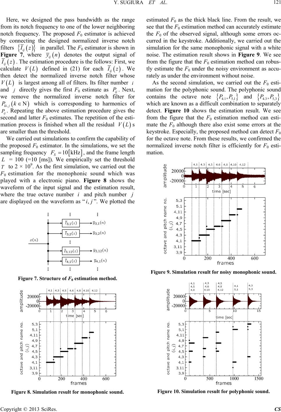
In this paper, we analyze an inverse notch filter and present its application to F0 (fundamental frequency) estimation.
The inverse notch filter is a narrow band pass filter and it has an infinite impulse response. We derive the explicit forms
for the impulse response and the sum of squared impulse response. Based on the analysis result, we derive a normalized
inverse notch filter whose pass band area is identical to unit. As an application of the normalized inverse notch filter, we
propose an F0 estimation method for a musical sound. The F0 estimation method is achieved by connecting the normal-
ized inverse notch filters in parallel. Estimation results show that the proposed F0 estimation method effectively detects
F0s for piano sounds in a mid-range.
Keywords: Band Pass Filter; Inverse Notch Filter; Impulse Response Analysis
1. Introduction
In speech processing, image processing, biomedical sig-
nal processing, and many other signal processing fields,
it is important to eliminate the narrowband signal. The
examples of the narrowband signal are a hum noise from
the power supply, an acoustic feedback, and an interfere-
ence noise, and so on. A notch filter is useful for the
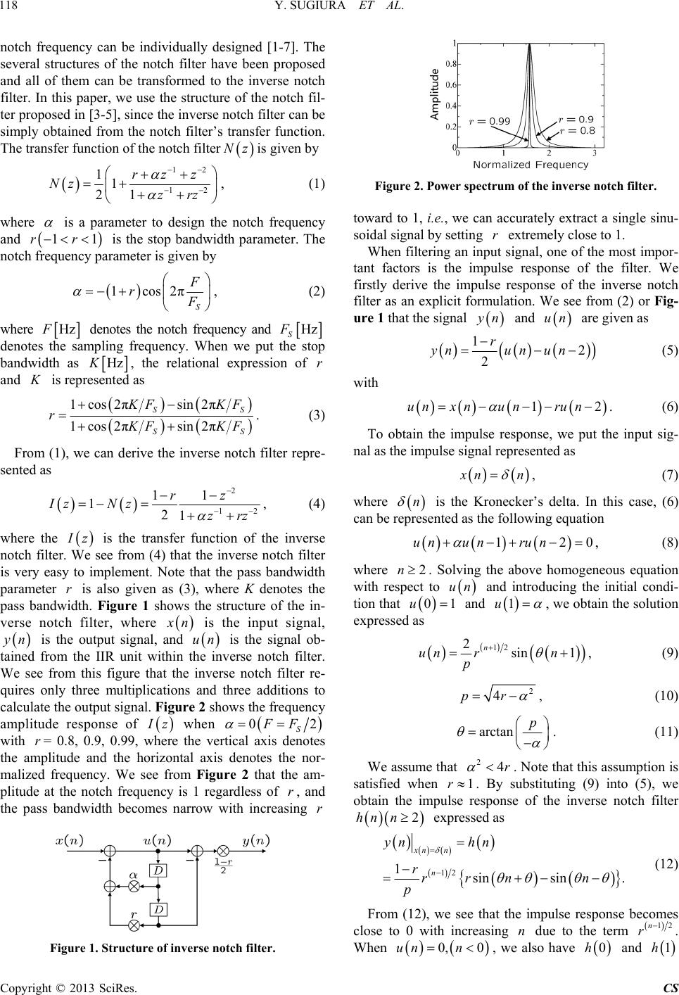
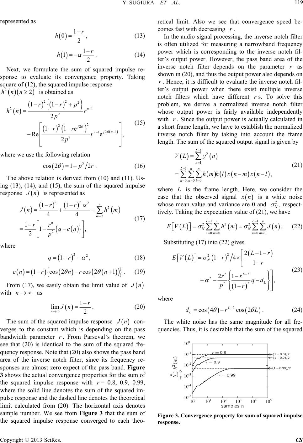
elimination of the narrowband signal [1-7], where the
notch filter passes all frequencies expect of a stop fre-
quency band centered on a center frequency, called as the
notch frequency. The notch filter has a simple structure,
and its stop bandwidth and its notch frequency are indi-
vidually designed. The notch filter is used in many ap-
plications and it has been analyzed in many literatures
[1,4-7].
On the other hand, an inverse notch filter is a band
pass filter which has the inverse characteristics of the
notch filter. In contrast to the notch filter, there are few
applications of the inverse notch filter. As an example of
the applications, an active noise control system for re-
ducing a sinusoidal noise has been proposed [8]. In this
system, the inverse notch filter is used to extract the si-
nusoidal noise. Unfortunately, the system is designed
without respect to the impulse response of the inverse
notch filter. Hence, the inverse notch filter cannot accu-
rately extract the sinusoidal noise when the filter output
is in the transient state. To utilize the inverse notch filter
more effectively for not only the active noise control
system but also many other applications, a more detail
analysis of the impulse response for the inverse notch
filter needs to be required.
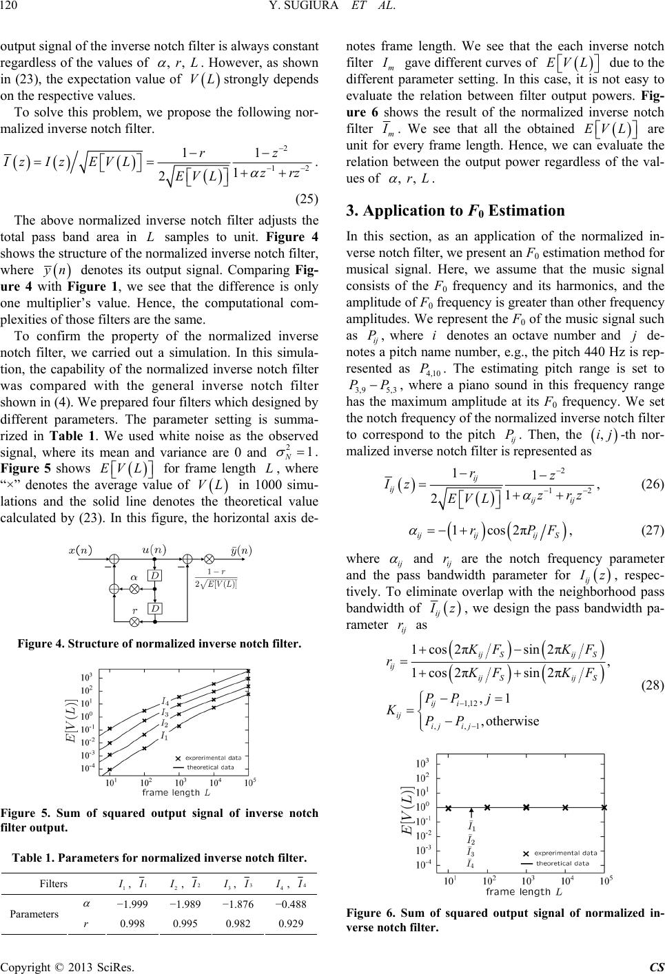
In this paper, we derive an explicit form for the infinite
impulse response of the inverse notch filter. Additionally,
we derive an explicit form for the sum of the squared
impulse response. Then, we reveal the limit values of
these two infinite sequences. Next, based on the analysis
results, we propose a normalized notch filter whose pass
band area is adjusted to unit. The normalized inverse
notch filter is efficient to estimate the output power in the
short time such as the frame processing. Finally, as an
application of the normalized inverse notch filter, we
present an F0 estimation method for a musical sound. In
the F0 estimation method, we use multiple normalized
inverse notch filters whose pass frequencies are identical
to F0s for each monophonic sound, respectively. These
normalized inverse notch filters are connected in parallel.
In the estimation procedure, we detect F0 from the in-
verse notch filter whose output power is largest among
all the inverse notch filter output powers. From the
simulation results, we see that the proposed F0 estimation
method can effectively detect the F0 both of for the
monophonic sounds and the polyphonic sounds.
2. Performance Analysis of Inverse Notch
Filter
In this section, we explain both of the notch filter and the
inverse notch filter, where the latter filter has an inverse
characteristic of the notch filter. The notch filter passes
all frequencies expect of the narrow frequency band cen-
tered on the notch frequency. The stop bandwidth and the
C
opyright © 2013 SciRes. CS

Y. SUGIURA ET AL.
118
notch frequency can be individually designed [1-7]. The
several structures of the notch filter have been proposed
and all of them can be transformed to the inverse notch
filter. In this paper, we use the structure of the notch fil-
ter proposed in [3-5], since the inverse notch filter can be
simply obtained from the notch filter’s transfer function.
The transfer function of the notch filteris given by

Nz

12
12
rzz
zrz




 



11
21
Nz , (1)
where

is a parameter to design the notch frequency
and is the stop bandwidth parameter. The
notch frequency parameter is given by

11rr 

1cos2π
S
F
r
F
  



, (2)
where

HzF denotes the notch frequency and


HzF

S
denotes the sampling frequency. When we put the stop
bandwidth as

HzK r, the relational expression of
and is represented as
K


1cos2π
1cos2π
sin 2π
sin 2π
SS
SS
K
FKF
r
K
FKF

. (3)
From (1), we can derive the inverse notch filter repre-
sented as
 
2
12
11rz
zrz 





121 Iz Nz , (4)
where the
I
z
r
is the transfer function of the inverse
notch filter. We see from (4) that the inverse notch filter
is very easy to implement. Note that the pass bandwidth
parameter is also given as (3), where K denotes the
pass bandwidth. Figure 1 shows the structure of the in-
verse notch filter, where


x
n

is the input signal,

y
n

un
is the output signal, and is the signal ob-
tained from the IIR unit within the inverse notch filter.
We see from this figure that the inverse notch filter re-
quires only three multiplications and three additions to
calculate the output signal. Figure 2 shows the frequency
amplitude response of

I
z when

02FF
r
rr
S
with = 0.8, 0.9, 0.99, where the vertical axis denotes
the amplitude and the horizontal axis denotes the nor-
malized frequency. We see from Figure 2 that the am-
plitude at the notch frequency is 1 regardless of , and
the pass bandwidth becomes narrow with increasing

Figure 1. Structure of inverse notch filter.
Figure 2. Power spectrum of the inverse notch filter.
toward to 1, i.e., we can accurately extract a single sinu-
soidal signal by setting extremely close to 1.
r
When filtering an input signal, one of the most impor-
tant factors is the impulse response of the filter. We
firstly derive the impulse response of the inverse notch
filter as an explicit formulation. We see from (2) or Fig-
ure 1 that the signal


y
n

un

and are given as
  
12
2
r
ynun un


(5)
with






12un xnunrun 

. (6)
To obtain the impulse response, we put the input sig-
nal as the impulse signal represented as




x
nn  , (7)


where n
 is the Kronecker’s delta. In this case, (6)
can be represented as the following equation




120un unrun 

 
2n
, (8)
where . Solving the above homogeneous equation
with respect to


un and introducing the initial condi-
tion that


01u


1u

and



, we obtain the solution
expressed as



12
2sin 1
n
un rn
p

, (9)


2
4pr

, (10)
arctan p 





24r

. (11)
We assume that

. Note that this assumption is
satisfied when 1r

. By substituting (9) into (5), we
obtain the impulse response of the inverse notch filter




2hn n expressed as




 



12
1sinsin .
xn n
n
yn hn
rrrn n
p








n

(12)
From (12), we see that the impulse response becomes
close to 0 with increasing due to the term 12n r.
When






0, 0un n


1h 0h and , we also have


Y. SUGIURA ET AL. 119
represented as

1
02
r
h

, (13) 

1
12
r



 
22hnn
h. (14)
Next, we formulate the sum of squared impulse re-
sponse to evaluate its convergence property. Taking
square of (12), the squared impulse response
is obtained as
 




1
21
1e ,
jn
n
r
 







22
2
2
2
2
22
2
11
2
11e
Re 2
n
j
rrp
hn r
p
rr
p










(15)
where we use the following relation
2
1 2pr

cos 2  . (16)
The above relation is derived from (10) and (11). Us-
ing (13), (14), and (15), the sum of the squared impulse
response
J
n is represented as
 
 
 
22
2
2
11
44
11,
2
n
rr 2
2
n
m
J
n
rr
qcn
p
 






hm




22
1qr
(17)
where

 
  

cos2 1n  
, (18)
 
1cos2cnrn r   . (19)
From (17), we easily obtain the limit value of


J
n
n

with as
1
2
r
Jn  lim
n . (20)
The sum of the squared impulse response


J
n
r
r
r
r
r
r
r
 
 
12
1
1
000
,
L
n
Lnn
nml
VLy n
hmhlxnmxn l





con-
verges to the constant which is depending on the pass
bandwidth parameter . From Parseval’s theorem, we
see that (20) is identical to the sum of the squared fre-
quency response. Note that (20) also shows the pass band
area of the inverse notch filter, since its frequency re-
sponses are almost zero expect of the pass band. Figure
3 shows the actual convergence properties for the sum of
the squared impulse response with = 0.8, 0.9, 0.99,
where the solid line denotes the sum of the squared im-
pulse response and the dashed line denotes the theoretical
limit calculated from (20). The horizontal axis denotes
sample number. We see from Figure 3 that the sum of
the squared impulse response converged to each theo-
retical limit. Also we see that convergence speed be-
comes fast with decreasing .
In the audio signal processing, the inverse notch filter
is often utilized for measuring a narrowband frequency
power which is corresponding to the inverse notch fil-
ter’s output power. However, the pass band area of the
inverse notch filter depends on the parameter as
shown in (20), and thus the output power also depends on
. Hence, it is difficult to evaluate the inverse notch fil-
ter’s output power when there exist multiple inverse
notch filters which have different s. To solve this
problem, we derive a normalized inverse notch filter
whose output power is fairly available independently
with . Since the output power is actually calculated in
a short frame length, we have to establish the normalized
inverse notch filter by taking into account the frame
length. The sum of the squared output signal is given by




L

(21)
where is the frame length. Here, we consider the
case that the observed signal
x
n
2
is a white noise
whose mean value and variance are 0 and
N

, respect-
tively. Taking the expectation value of (21), we have
 
11
22 2
00 00
Ln Ln
NN
nm nm
EVLh mJn 

 

 
 
. (22)
Substituting (17) into (22) gives


2
2
22
2
22
21
141
21 ,
1
N
L
L
Lr
EVL rr
rr
qd
pr



 
  
 

 (23)





 







where


2
cos 4cos 2
L
L
drL



 . (24)
The white noise has the same magnitude for all fre-
quencies. Thus, it is desirable that the sum of the squared
Figure 3. Convergence property for sum of squared impulse
response.

Y. SUGIURA ET AL.
120
output signal of the inverse notch filter is always constant
regardless of the values of , , rL

. However, as shown
in (23), the expectation value of strongly depends
on the respective values.

VL
To solve this problem, we propose the following nor-
malized inverse notch filter.
 
2
12
11rz
zrz


1
2
Iz Iz EVLEVL




L


 

.
(25)
The above normalized inverse notch filter adjusts the
total pass band area in samples to unit. Figure 4
shows the structure of the normalized inverse notch filter,
where

y
n denotes its output signal. Comparing Fi g-
ure 4 with Figure 1, we see that the difference is only
one multiplier’s value. Hence, the computational com-
plexities of those filters are the same.
To confirm the property of the normalized inverse
notch filter, we carried out a simulation. In this simula-
tion, the capability of the normalized inverse notch filter
was compared with the general inverse notch filter
shown in (4). We prepared four filters which designed by
different parameters. The parameter setting is summa-
rized in Table 1. We used white noise as the observed
signal, where its mean and variance are 0 and N
21


.
Figure 5 shows for frame length , where
“×” denotes the average value of in 1000 simu-
lations and the solid line denotes the theoretical value
calculated by (23). In this figure, the horizontal axis de-

EVL 
L 

VL
Figure 4. Structure of normalized inverse notch filter.
Figure 5. Sum of squared output signal of inverse notch
filter output.
Table 1. Parameters for normalized inverse notch filter.
Filters 1
I
, 1 I 2
I
, 2 I 3
I
, 3 I4
I
, 4 I

−1.999 −1.989 −1.876 −0.488
Parameters
notes frame length. We see that the each inverse notch
filter m
I
gave different curves of  due to the
different parameter setting. In this case, it is not easy to
evaluate the relation between filter output powers. Fig-
ure 6 shows the result of the normalized inverse notch
filter

EVL

m

I
. We see that all the obtained

EVL

, , rL

are
unit for every frame length. Hence, we can evaluate the
relation between the output power regardless of the val-
ues of

.
3. Application to F0 Estimation
In this section, as an application of the normalized in-
verse notch filter, we present an F0 estimation method for
musical signal. Here, we assume that the music signal
consists of the F0 frequency and its harmonics, and the
amplitude of F0 frequency is greater than other frequency
amplitudes. We represent the F0 of the music signal such
as ij , where denotes an octave number and de-
notes a pitch name number, e.g., the pitch 440 Hz is rep-
resented as 4,10. The estimating pitch range is set to
3,9 5,3
Pij
P
PP

, where a piano sound in this frequency range
has the maximum amplitude at its F0 frequency. We set
the notch frequency of the normalized inverse notch filter
to correspond to the pitch ij. Then, the -th nor-
malized inverse notch filter is represented as
P

,ij
 
r 0.998 0.995 0.982 0.929
2
12
11
1
2
ij
ij
ij ij
rz
Iz zrz
EVL







, (26)


1cos2π
ijijij S
rPF   , (27)
where ij

and ij r are the notch frequency parameter
and the pass bandwidth parameter for ij

I
z, respec-
tively. To eliminate overlap with the neighborhood pass
bandwidth of


ij
I
z
ij
r, we design the pass bandwidth pa- rameter as



1,12
,,1
1cos2πsin 2π
,
1cos2πsin 2π
,1
,otherwise
ij Sij S
ij
ij Sij S
ij i
ij ij ij
KF KF
rKF KF
PP j
KPP










(28)
Figure 6. Sum of squared output signal of normalized in-
verse notch filter.

Y. SUGIURA ET AL. 121
Here, we designed the pass bandwidth as the range
from its notch frequency to one of the lower neighboring
notch frequency. The proposed F0 estimator is achieved
by connecting the designed normalized inverse notch
filters
 
ij
I
z in parallel. The F0 estimator is shown in
Figure 7, where

ij
y
n denotes the output signal of

ij
I
z. The estimation procedure is the follows: First, we
calculate defined in (21) for each

VL


ij
I
z

VL i
. We
then detect the normalized inverse notch filter whose
is largest among all of filters. Its filter number
and

j
directly gives the first F0 estimate as ij . Next,
we remove the normalized inverse notch filter for
,j which is corresponding to harmonics of
ij . Repeating the above estimation procedure gives the
second and latter F0 estimates. The repetition of the esti-
mation process is finished when all the residual
P

Pk
ki
P


VL

s
are smaller than the threshold.
We carried out simulations to confirm the capability of
the proposed F0 estimator. In the simulations, we set the
sampling frequency

10 kHzF
L
T
ij
,j
S, and the frame length
= 100 (=10 [ms]). We empirically set the threshold
to 2 × 109. As the first simulation, we carried out the
F0 estimation for the monophonic sound which was
played with a electronic piano. Figure 8 shows the
waveform of the input signal and the estimation result,
where the true octave number and pitch number
are displayed on the waveform as “i”. We plotted the
Figure 7. Structure of F0 estimation method.
Figure 8. Simulation result for monophonic sound.
estimated F0 as the thick black line. From the result, we
see that the F0 estimation method can accurately estimate
the F0 of the observed signal, although some errors oc-
curred in the keystroke. Additionally, we carried out the
simulation for the same monophonic signal with a white
noise. The estimation result shows in Figure 9. We see
from the figure that the F0 estimation method can robus-
tly estimate the F0 under the noisy environment as accu-
rately as under the environment without noise.
As the second simulation, we carried out the F0 esti-
mation for the polyphonic sound. The polyphonic sound
contains the octave note

4.1 5,1 and

,PP


,PP
4.35,3
which are known as a difficult combination to separately
detect. Figure 10 shows the estimation result. We see
from the figure that the F0 estimation method can esti-
mate the F0 although there also exist some errors at the
keystroke. Especially, the proposed method can detect F0
for the octave note. From these results, we confirmed the
normalized inverse notch filter is efficiently for F0 esti-
mation.
Figure 9. Simulation result for noisy monophonic sound.
Figure 10. Simulation result for polyphonic sound.

Y. SUGIURA ET AL.
122
4. Conclusion
In this paper, we analyzed the inverse notch filter and
derived the explicit forms for the impulse response and
the sum of squared impulse response. Based on the
analysis result, we derived a normalized inverse notch
filter whose pass band area is identical to unit to evaluate
the output powers between the multiple inverse notch
filters which have different parameters. Moreover, we
established an F0 estimator by connecting the normalized
inverse notch filters in parallel. Estimation results
showed that the proposed F0 estimator effectively detects
F0s for electronic piano sound in a mid-range.
REFERENCES
[1] A. Nehorai, “A Minimal Parameter Adaptive Notch Filter
with Constrained Poles and Zeros,” IEEE Transactions
on Acoustics, Speech and Signal Processing, Vol. 33, No.
4, 1985, pp. 983-996. doi:10.1109/TASSP.1985.1164643
[2] H. C. Chong and U. L. Sang, “Adaptive Line Enhance-
ment by Using an IIR Lattice Notch Filter,” IEEE Trans-
actions on Acoustics, Speech and Signal Processing, Vol.
37, No. 4, 1989, pp. 585-589. doi:10.1109/29.17543
[3] C. C. Tseng and S. C. Pei, “IIR Multiple Notch Filter
Design Base on Allpass Filter,” IEEE Transactions on
Circuits and Systems II: Analog and Digital Signal Proc-
essing, Vol. 44, No. 2, 1997, pp. 133-136.
[4] S. C. Pei, W. S. Lu and C. C. Tseng, “Analytical Two-
Dimensional IIR Notch Filter Design Using Outer Prod-
uct Expansion,” IEEE Transactions on Circuits and Sys-
tems II: Analog and Digital Signal Processing, Vol. 44,
No. 9, 1997, pp. 765-768.
[5] Y. V. Joshi and S. C. D. Roy, “Design of IIR Multiple
Notch Filters Based on All-Pass Filters,” IEEE Transac-
tions on Circuits and Systems II: Analog and Digital Sig-
nal Processing, Vol. 46, No. 2, 1999, pp. 134-138.
[6] M. Goto, “A Real-Time Music-Scene-Description System:
Predominant-F0 Estimation for Detecting Melody and
Bass Lines in Real-World Audio Signals,” Speech Com-
munication, Vol. 43, No. 4, 2004, pp. 311-329.
doi:10.1016/j.specom.2004.07.001
[7] V. DeBrunner, “An Adaptive, High-Order, Notch Filter
Using All Pass Sections,” IEEE International Conference
on Acoustics, Speech and Signal Processing, Vol. 3, Seat-
tle, 12-15 May 1998, pp. 1477-1480.
[8] Y. Xiao, “A New Efficient Narrowband Active Noise
Control System and Its Performance Analysis,” IEEE
Transactions on Audio, Speech, and Language Process-
ing, Vol. 19, No. 7, 2011, pp. 1865-1874.
doi:10.1109/TASL.2010.2101598