Applied Mathematics, 2010, 1, 344-350
doi:10.4236/am.2010.15045 Published Online November 2010 (http://www.SciRP.org/journal/am)
Further Properties of Reproducing Graphs
Jonathan Jordan, Richard Southwell
School of Mathematics and Statistics, University of Sheffield, Sheffield, United Kingdom
Received July 30, 2010; revised September 16, 2010; accepted September 18, 2010
Abstract
Many real world networks grow because their elements get replicated. Previously Southwell and Cannings
introduced a class of models within which networks change because the vertices within them reproduce. This
happens deterministically so each vertex simultaneously produces an offspring every update. These offspring
could represent individuals, companies, proteins or websites. The connections given to these offspring de-
pend upon their parent’s connectivity much as a child is likely to interact with their parent’s friends or a new
website may copy the links of pre-existing one. In this paper we further investigate one particular model,
‘model 3’, where offspring connect to their parent and parent’s neighbours. This model has some particularly
interesting features, including a degree distribution with an interesting fractal-like form, and was introduced
independently under the name Iterated Local Transitivity by Bonato et al. In particular we show connections
between this degree distribution and the theory of integer partitions and show that this can be used to explain
some of the features of the degree distribution; we give exact formulae for the number of complete subgraphs
and the global clustering coefficient and we show how to calculate the minimal cycle basis.
Keywords: Reproduction, Graph, Network, Deterministic
1. Introduction
Networks are everywhere; wherever a system can be
thought of as a collection of discrete elements, linked up
in some way, networks occur. With the acceleration of
information technology more and more attention is being
paid to the structure of these networks, and this has led to
the proposal of many models, for example Erdős-Rényi
random graphs [1], preferential attachment graphs [2,3],
random geometric graphs [4], and small world graphs
[5].
In many situations networks grow − they expand in
size as material is produced from the inside, not added
from outside. To study network growth, in [6-8] Southwell
and Cannings introduced a class of pure reproduction
models, where networks grow because the vertices
within reproduce. These models have some similarities
to duplication models such as those analysed in [9,10],
but in those models only one vertex (chosen randomly)
reproduces at every update, whereas in our models every
vertex reproduces at every time step.
We suggest that our models, or variations on them, can
be applied to many situations where entities are intro-
duced which derive their connections from pre-existing
elements. Most obviously they could be used to model
social networks, collaboration networks, networks within
growing organisms, the internet and protein-protein
interaction networks. The model also captures aspects of
the way collaboration networks change over time, with
new students collaborating with their supervisors and the
people their supervisor collaborates with.
In this paper we focus upon the dynamics of one of
these eight pure reproduction models - labelled ‘model 3’
by the labelling in [7]. In this model, a graph is updated
by simultaneously giving each vertex an offspring which
is born connected to its parent and its parent’s neigh-
bours. This model was introduced independently in [11]
under the name of Iterated Local Transitivity (ILT),
proposed as a model for the growth of online social
networks. The model has some very interesting mathe-
matical properties, most particularly its degree distri-
bution which has an intricate fractal-like form despite
being generated by a simple recursion.
In this paper we study this degree distribution and
reveal connections with the theory of integer partitions,
which allows some of the features of the degree
distribution to be explained. We also derive exact form-
ulae for the number of complete graphs and the global
clustering coefficient, which we compare with the
asymptotic results on the local clustering coefficient in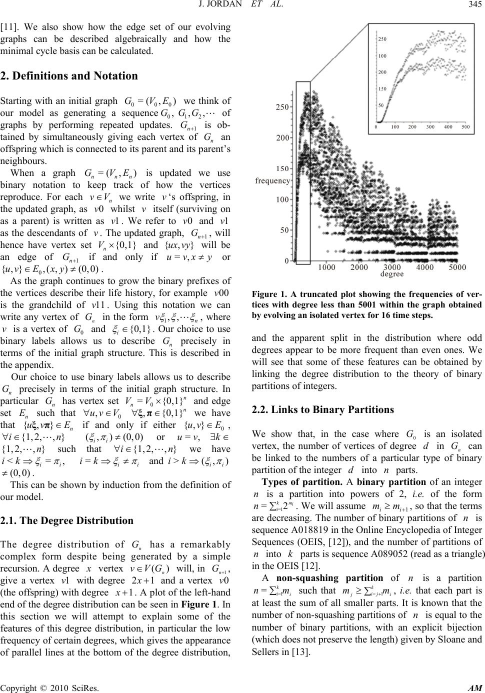

J. JORDAN ET AL. 345
[11]. We also show how the edge set of our evolving
graphs can be described algebraically and how the
minimal cycle basis can be calculated.
2. Definitions and Notation
Starting with an initial graph 000 =( ,)GVE we think of
our model as generating a sequence0,G12 ,,GG of
graphs by performing repeated updates. 1n G

is ob-
tained by simultaneously giving each vertex of n G an
offspring which is connected to its parent and its parent’s
neighbours.
When a graph =( ,)
nnn
GVE is updated we use
binary notation to keep track of how the vertices
reproduce. For each n vV we write v‘s offspring, in
the updated graph, as 0v whilst v itself (surviving on
as a parent) is written as 1v. We refer to 0v and 1v
as the descendants of v. The updated graph, 1n G

, will
hence have vertex set {0,1}
n
V and {,}ux vy will be
an edge of 1n G if and only if =,uvxy

or
0
{,},(, )(0,0)uvExy.
As the graph continues to grow the binary prefixes of
the vertices describe their life history, for example 00v
is the grandchild of 11v. Using this notation we can
write any vertex of n G in the form 1,, n v

 , where
v is a vertex of 0 G and {0,1}
i


. Our choice to use
binary labels allows us to describe n G precisely in
terms of the initial graph structure. This is described in
the appendix.
Our choice to use binary labels allows us to describe
n
G precisely in terms of the initial graph structure. In
particular n G has vertex set 0
={0,1}
n
n
VV and edge
set n E such that 0 ,uvV ,{0,1}
n
ξπ we have
that {, }n uv Eξπ if and only if either 0 {,}uv E

,
{1, 2,,}in  (, )(0,0)
ii

  or =,uv k


{1, 2,,}n such that {1, 2,,}in  we have
<=,
ii
ik

  =ii ik

  and>(,)
ii
ik

 
(0,0).
This can be shown by induction from the definition of
our model.
2.1. The Degree Distribution
The degree distribution of n G has a remarkably
complex form despite being generated by a simple
recursion. A degree
x
vertex )( n GVv  will, in 1n G,
give a vertex 1v with degree 12x and a vertex 0v
(the offspring) with degree 1

x. A plot of the left-hand
end of the degree distribution can be seen in Figure 1. In
this section we will attempt to explain some of the
features of this degree distribution, in particular the low
frequency of certain degrees, which gives the appearance
of parallel lines at the bottom of the degree distribution,
Figure 1. A truncated plot showing the frequencies of ver-
tices with degree less than 5001 within the graph obtained
by evolving an isolated vertex for 16 time steps.
and the apparent split in the distribution where odd
degrees appear to be more frequent than even ones. We
will see that some of these features can be obtained by
linking the degree distribution to the theory of binary
partitions of integers.
2.2. Links to Binary Partitions
We show that, in the case where 0 G is an isolated
vertex, the number of vertices of degree d in n G can
be linked to the numbers of a particular type of binary
partition of the integer d into n parts.
Types of partition. A binary partition of an integer
n is a partition into powers of 2, i.e. of the form
i
m k
i
n2= 1=
. We will assume 1
ii mm, so that the terms
are decreasing. The number of binary partitions of n is
sequence A018819 in the Online Encyclopedia of Integer
Sequences (OEIS, [12]), and the number of partitions of
n into k parts is sequence A089052 (read as a triangle)
in the OEIS [12].
A non-squashing partition of n is a partition
i
k
imn 1=
= such that i
k
ji
jmm 
1= , i.e. that each part is
at least the sum of all smaller parts. It is known that the
number of non-squashing partitions of n is equal to the
number of binary partitions, with an explicit bijection
(which does not preserve the length) given by Sloane and
Sellers in [13].

J. JORDAN ET AL. 346
A similar idea to non-squashing partitions is that of a
strongly decreasing partition, defined by Olsson in
[14], which requires a strict inequality: =1 >k
j
i
ij
mm

.
We will define a non-jumping binary partition to be
a binary partition with the restriction that =1
k
m and
that 11
ii
mm

, i.e. that all integer powers of 2 less
than 1
2m are represented in the partition.
2.3. Recurrences for Partitions and the Degree
Distribution
We link the degree distribution to two types of partition,
strongly decreasing partitions and the non-jumping
binary partitions defined above.
Theorem 1 Let 0 G be an isolated vertex. Then
1) The number of vertices of degree d in n
G is
twice the number of non-jumping binary partitions of d
into n parts.
2) The total number of vertices of degree d in all
graphs ,1
i
Gi, is twice the number of strongly de-
creasing partitions of d (which is equal to the number
of non-jumping binary partitions of d).
Proof: To see this, we show that a bijection between
the sets of strongly decreasing partitions and non-
jumping binary partitions is naturally related to the
representation of the vertices in the form 12 n v

 .
The idea of the bijection is essentially the same as that
for binary partitions and non-squashing partitions given
by Sloane and Sellers in [13].
Let 11 =pq be the partition of 1 given by 1
(which is both a non-jumping binary partition and a
strongly decreasing partition). This partition corresponds
to the two vertices of degree 1 in 1 G. We then proceed
inductively: we assume that we have a non-jumping
binary partition
j
p of length j and sum
x
and a
strongly decreasing partition
j
q with sum
x
. Then if
1=0 j

, form a non-jumping binary partition 1
j
p

with sum 1
x
 and length 1j

from
j
p by adding a
new 1 part on the end, and form a new strongly
decreasing partition 1
j
q with sum 1
x
 by adding 1
to the largest part of j q. If 1=1
j

, form 1
j
p

by
doubling every part of
j
p and adding a new 1 part on
the end, giving a non-jumping binary partition with sum
21
x
 and length 1j, and form 1
j
q by adding a
new part on the beginning of
j
q whose size is the
minimum possible, i.e., 1
x

, giving a strongly
decreasing partition with sum 21
x
.
We now show that by working backwards it can be
seen that each partition of each type arises in exactly one
way from a sequence of ,2
jjn

. If we have a
non-jumping binary partition
j
p with exactly one 1
part, set =1
j

and form 1
j
p by removing the 1
part and dividing the remaining parts by 2; if
j
p has
more than one 1 part set =0
j

and form 1
j
p

by
simply removing one 1 part. If we have a strongly
decreasing partition
j
q such that the largest part is
equal to one more than the sum of the remaining parts,
set =1
j

and form 1
j
q

by removing the largest part;
otherwise the largest part will be larger than this, and we
can set =0
j

and form 1
j
q by subtracting one from
the largest part.
As each sequence of ,2
jjn

 corresponds to a
pair of vertices of n G with the same degree (one with
1=0

and one with 1=1

) this shows that the number
of vertices with degree d in n G is twice the number
of non-jumping binary partitions of d into n parts.
The second part follows from the bijection between
non-jumping binary partitions of d and strongly de-
creasing partitions of d.
The total number of strongly decreasing partitions of
d (of any length), and hence also the number of
non-jumping binary partitions of any length, is sequence
A040039 in the OEIS, [12] (this can be seen by using the
above recurrence). Hence, with appropriate modification
based on the initial graph, this also gives the total
number of vertices of degree d in all graphs n G in
total; as mentioned above if we start with an isolated
vertex then A040039 needs to be doubled to give the
right values, as 1 G contains two vertices of degree 1.
Features of the degree distribution. The plot of the
degree distribution of n G has a number of distinctive
features. We attempt to use the connection to binary
partitions to explain some of these, starting with the first
n
G which contains vertices of degree d. Throughout
this section we will assume that 0 G is an isolated
vertex, so the results of Theorem 1 apply without
modification. We start by finding the first graph n G
which contains a vertex of degree d.
Proposition 2 Write d in the form sd r12=
for some integers
r
and
s
such that r s2<0. Then
the smallest n such that d occurs as a degree in n G
is
r
plus the number of ones in the binary
representation of
s
, that is m
r
msr 
1
0= , where m
s is
the digit corresponding to m 2 in the binary
representation of
s
.
Proof. Given d, the shortest non-jumping binary
partition of d can have at most two occurrences of
each power of 2. (If m 2 occurs three times, replace
them by mm 22 1

 to obtain a shorter non-jumping
binary partition.) A unique shortest non-jumping binary
partition of d can then be found by writing
sd r12= for some integers
r
and
s
such that
0<2,
r
sand forming the partition m
m
r
msd 1)2(= 1 0= 
.
Hence the smallest n for which sd r12= is a
possible value of n X is
r
plus the number of ones in

J. JORDAN ET AL. 347
the binary representation of
s
, that is m
r
msr 
1
0= .
Then d occurs as a degree for the first time in
1
=0
r
rs
m
m
G
, with multiplicity 2 (as 1
G contains two
vertices of degree 1).
We note that the stage at which d appears for the
first time is given by A0147011)( d from the OEIS,
[12]. Furthermore, the smallest d which appears as a
degree for the first time in r G2 will be 221

r, for
which all digits of
s
are 1, and similarly, the smallest
d which appears as a degree for the first time in 12 r G
will be 223=222 11  rrr . These numbers give
sequence A027383 in the OEIS.
We now show that arguments involving values
sd r12= with small numbers of zeros in the binary
representation of
s
, explain certain features of the plot
of the degree distribution. The first part of the following
proposition applies to n G with even n, and the second
part to n G with odd n.
Proposition 3
1) If 222= 1
tr
d for some 2<0  rt , there
will be 2)2(r vertices with degree d in r G2, and if
32= 1
r
d or 222= 11  rr d there will be 1)2(

r
vertices with degree d in r G2.
2) If 2223= 1 tr
d for some 2<0

rt , there
will be 2)2(r vertices with degree d in 12 r G, and
if 323=1 r
d or 222= 1 r d there will be
1)2( r vertices with degree d in 12 r G.
Proof. If 222= 1
tr
d for some 1

rt then
12=
1
0= 

rsr m
r
m, so d appears as a degree for the
first time in 12 r G. We can also consider the number of
non-jumping binary partitions of d of length
r
2:
these can be obtained by taking the partition
m
m
r
msd 1)2(=1 0= 
 and replacing one part of size m
2
by two of size 1 2m, as long as either 1=
m
s or
1=rt so that the non-jumping definition is met. As
1=
m
s unless
t
m=, there will be 2

r
such
partitions, or 1
r
in the cases 0=t and 1=

rt , so
if 1
G has two vertices of degree 1 these degrees will
have multiplicity 2)2(r or 1)2(r, giving the first
part.
Similarly, if 2223= 1 tr d there will be 2

r
non-jumping binary partitions of length 12 
r
, or 1

r
in the cases 0=t and 1=

rt .
Similar arguments can also be constructed involving
values sd r12= with other small numbers of zeros
in the binary representation of
s
.
2.4. The Degree Distribution and Markov Chains
We note that we can choose a random vertex in each n G
by choosing a random vertex v of 0 G and defining a
sequence of independent Bernoulli(1/2) random
variables ii)(

; we then let our random vertex be the
vertex with label 12 n
v
 
. We can then obtain the
degree of our random vertex in n G by letting 0 X be
the degree of a random vertex in 0
G and=
i
X
1
(1)1
ni i
X



, and nn X)( can then be considered as
a Markov chain on the non-negative integers.
We note that if we let mXY nn mod= then nn Y)(
is a Markov chain on a finite state space {0,1, ,1}m

.
The most interesting cases are where m is a power of
2; for example if 2=m the transition matrix is








1/21/2
10
with stationary distribution (1/3,2/3) , implying that the
probability that n
X is odd, and hence the proportion of
vertices of n G with odd degree, converges to 2/3 as

n. Similar results can be obtained for n X modulo
m Stationary distribution
2 1(1, 2)
3
4 1(3,4,2,6)
15
8 1(29, 40,20, 44, 22, 28,14,58)
255
other powers of 2, but if we work with n
X
modulo an
odd prime the transition matrix is doubly stochastic and
so we get a uniform distribution as the stationary dis-
tribution.
2.5. Lognormal Limit
In this section we discuss some asymptotic properties of
the degree distribution. It is shown in [11] that asym-
ptotically the distribution has “binomial-type’’ behaviour,
in the sense that n
j



nodes have degree around j 2,
which also implies that the degree distribution has a
roughly lognormal form for large n; the following
result goes a bit further.
Theorem 4
As

n, we have
1) with probability 1,
);2(log=)(1log
log
1
  
n
Xn
2) (0,1).
)2(log
)2(loglog N
n
nX
d
n

Proof: For 1n, we can write












 1
log)(1log)(log=)(log
1
1
11
n
n
nnn X
X
XX


J. JORDAN ET AL. 348
1
1
1
= log()log(1)log11
nn
n
XX 



 



1
=2
1
=log(1)log1.
1
n
j
jj
X




 







This, applying the Strong Law of Large Numbers to
)(1log
1
2= j
n
j
 
, is enough to show that
)2(log)/(log
liminf   nX n n, almost surely. Hence,
for any )2(log<a we have 1
>1
n
n
a
Xa

 for n
large enough, and so
11
=2 =2
11
log 1<log 1
111
1
nn
j
jj
j
C
Xa
a



 








 

for some C depending on a.
Note that if 1=
1
z and 1=
1 nnazz then
1
1
=2
1
log=loglog 1,
1
n
n
jj
zna z









but 1
1
=

a
a
z
n
n, so
11
=2
1
log1= log(1)loglog(1)
11
1
nn
j
j
anaa
a
a



 




 

<log .
1
a
a




Hence =2
1
log 1=
1
j
j
Y
X








, say, is finite, and we
can write
,)(1log=log 1
1
2=
1


nj
n
j
nYX
 with  YYn. Hence the
Strong Law of Large Numbers tells us that, almost
surely,
),2(log=)(1log
log
1
  
n
Xn
and the Central Limit Theorem tells us that
loglog( 2)(0,1).
log(2)
n
d
Xn N
n

2.6. Number of Complete Graphs
The following theorem gives an exact formula for )(n
m
k,
the number of m vertex complete graphs in n
G, in
terms of the number of complete graphs of various sizes
within the initial graph.
Theorem 5
() (0)
=1 =1
11
=(1) (1)
11
mh
nn mh
mi
hi
mh
kh k
hi


 

 
 

 

Proof. Suppose the subgraph of n
G induced upon
some n
X
V is an m vertex complete graph. In the
updated graph 1n G there will be several complete
graphs which are induced upon the descendants
{0,1}

X of vertices from
X
. In particular there will
be m complete graphs on 1m vertices (one induced
upon }:1{0}{ Xuuv

 for each Xv ) together with
1

m complete graphs on m vertices (one induced
upon }:1{ Xuu

and one induced upon
}}{:1{0}{ vXuuv


 for each Xv).
We will now show that every m vertex complete
graph in 1n
G can be constructed in the above manner.
Suppose there is an m vertex complete graph in 1n
G
induced upon 1 n VY . Let n VX be minimal such
that each vertex of
Y
is descended from a vertex of
X
.
The subgraph of n
G induced upon
X
must be a
complete graph since if it were not then a pair of its
descendants in
Y
would not be linked. Since mY|=| ,
we have mX

|| . Offspring of distinct vertices in
X
are not adjacent, this means there can be at most one
Xv

such that Xv

0. This implies 1||

mX ,
and also that }:1{= XuuY

or
}}{:1{0}{= vXuuvY


 for some Xv.
We have hence shown that the number, )( n
m
k, of m
vertex complete graphs in n G satisfies the difference
equation (1)()()
1
=( 1)( 1)
nnn
mmm
kmkmk


.
This system can be solved using linear algebra by
writing
(1)(1)(1)()
12
=(,,)=
nnnT n
kkk Mk

where the infinite matrix
M
is such that 0=
,ji
M
unless ji =, in which case 1=
,iM ji , or 1=

ji in
which case 1=
,

iM ji .
For 1h the hth eigenvalue of this matrix is
1)(=

h
h

, and the associated right eigenvector is
Thhheee ,...),(= )(
2
)(
1
)(
where
()
1(1)
=1
0
hi
h
i
iif hi
eh
otherwise










Solving
(0)( )
1
=h
h
h
ke 



we find that
(0)
=1
1
=.
1
h
hi
i
hk
i









J. JORDAN ET AL. 349
Expanding
()
1
()
hn
hh
h
e





yields the result.
2.7. Global Clustering Coefficient
The global clustering coefficient of n G is n
nn
P


where n  is the number of closed triplets (note that
each triangle gets counted as three closed triples) and n P
is the number of open triples in n G. We can describe the
global clustering coefficient in terms of the numbers of
vertices (0)
1
k, edges (0)
2
k, triangles (0)
3
k and open triples
0
P in the initial graph with the following result.
Theorem 6
The global clustering coefficient of n G is
  
 
(0)(0) (0)(0)(0)(0)
112122
(0)(0) (0)(0)(0)(0)
1121230
92 234 2
821235 41293
nnn
nn n
kkkkkk
kkkkkkP

 
Proof. First, ()
3
=3 n
nk
. We shall derive a recursion for
n
P. Let
x
be a vertex in n G; we shall describe the
open triples in 1n
G which terminate at a descendant of
.
x
Let ()={:{,} }
Ne nn
x
yV xy E be
x
’s neigh-
bourhood. Let ()
cl
x
be the set of n Ezy },{ such that
{,} ()
N
e
yz x (this corresponds to the set of closed
triplets containing
x
). Let ()
op
x
be the set of ),( zy
such that ()
N
e
yx and () ()
N
eNe
zy x

 (this cor-
responds to the set of open triplets terminating at
x
).
a) For ()
N
e
yx there will be one open triple
0}1,0,{ yxx in 1n G.
a’) For ()
N
e
yx there will be one open triple
0}1,0,{ yyx in 1n G.
b) For (,) () op yz x there will be one open triple
1}1,1,{ zyx in 1n G.
c) For (,) () op yz x there will be one open triple
0}1,0,{ zyx in 1n G.
d) For (,) () op yz x there will be one open triple
1}0,1,{ zyx in 1n G.
e) For (,) () op yz x there will be one open triple
1}1,0,{ zyx in 1n G.
e’) For (,) () op yz x there will be one open triple
0}1,1,{ zyx in 1n G.
f) For {,} ()
cl
yz x there will be one open triple
0}1,0,{ zyx in 1n G.
To see that every open triple
T
in 1n G which ter-
minates at a descendant of
x
will be of the type
a,a’,b,c,d,e,e’ or f note that every such
T
consists of
descendants of either 2 or 3 path connected vertices.
Suppose T consists of descendants of 2 path con-
nected vertices. There are two possibilities. T could
hold both descendants of
x
and one descendant y d of
()
N
e
yx

. In this case we must have 0=ydy because
the other possibility (1=yd y) implies that T is the
closed triple 1}1,0,{ yxx . So in this case we have that
0}1,0,{= yxxT is of type a. The other possibility is that
T holds one descendant x
d of
x
and both descen-
dants of ()
N
e
yx

; this implies T is of type a’. in a
similar way to before.
Suppose T consists of descendants of 3 path con-
nected vertices, then either 1) )(
o ),( x p zy such that
},,{=



zyxT or 2) {,}()
cl
yz x

 such that =T
{, ,}
x
yz

 , where {0,1},, 



.
Let us consider case 1). We must have (0,0)),(



and (0,0)),(



in order for T to be connected. Let
us consider the remaining possible values of


,( ,

).
When (1,1,1)=),,(



we have case b. When
(0,1,0)=),,(



we have case c. When
(1,0,1)=),,(



we have case d. When
(0,1,1)=),,(



we have case e. When
(1,1,0)=),,(



we have case e’. These are all the
possibilities under case 1).
Let us consider case 2). We require
1
},{},,{ 

n
Ezyyx




and 1 },{  n Ezy


. Again
we must have (0,0)),(



and (0,0)),(



in
order for T to be connected. In addition we require
0==


to ensure 1 },{  n Ezy


. These conditions
force (0,1,0)=),,(



, which is case f.
This means that we can enumerate the number of open
triples in 1n
G by counting the number of a,a’,b,c,d,e,e’
and f which are generated by each n
Vx . This yields
|| n E open triples of type a, || n E of type a’, n P of
type b, n
P of type c, n P of type d, n P of type e, n P
of type e’ and ()
3
=3 n
nk

 of type f.
This gives us the recursion ()
13
=2||53 n
nnn
PEPk

.
Adding this to the recursion from the proof of theorem 5
we gain the matrix equation
,
5320
0420
0031
0002
=)(
3
)(
2
)(
1
1
1)(
3
1)(
2
1)(
1














































n
n
n
n
n
n
n
n
P
k
k
k
P
k
k
k
which we can solve to find

(0) (0)(0)(0)(0)
121 230
4
=2 354.3
3
nn
n
Pkk kkkP

 



(0)
(0)(0) (0)
1
013
234 2,
3
n
n
kkkk 

and




()(0)(0) (0)(0)(0) (0)
3112 123
=22 342.
nn nn
kkkk kkk 

J. JORDAN ET AL. 350
Substituting these results into the formula,
()
3
()
3
3
3
n
n
n
k
kP


,
for the global clustering coefficient yields the stated
result.
The global clustering coefficient decreases asympto-
tically as n (4/5) making it smaller than the local clust-
ering coefficient, which decreases asymptotically as
n
(7/8) , as shown in [11].
2.8. Minimal Cycle Basis
A (simple) cycle of a graph ),(= EVG is a subset
EC such that the graph with vertex set
}},{,:{ Cvuvu  and edge set C is connected with
each vertex of degree 2.
The set )( cG yc of all cycles in a graph forms a
vector space with symmetric difference as addition.
When G is connected with a spanning tree T the
fundamental cycles of
T
form a cycle basis (that is, a
subset of )(
cG yc from which G can be generated).
The dimension )( cG yc is 1||||  VE ; a cycle basis
is minimal when it holds this many elements.
Theorem 7 If B is a minimal cycle basis of
),(= nnn EVG then
}},{:1}}1,{1},0,{0},1,{{{{1}= EvuuvvuuuBB



is a minimal cycle basis of ),(= 111  nnn EVG
Proof. ||2|=|1nn VV  and ||||3|=| 1nnn VEE 
 so
the dimension of the cycle space of 1n
G is ||2n E
plus the dimension of n G’s cycle space. This is equal to
the number of elements in B

because B consists of
the minimal cycle basis of B plus two triangles,
1}}1,{1},0,{0},1,{{ uvvuuu and
1}}1,{1},0,{0},1,{{ vuuvvv , for each edge n Evu

},{ .
Let
1}}1,{1},0,{0},1,{{= uvvuuu
be a triangle in B.  cannot be expressed as a linear
combinations of other elements from B since it holds
an edge 1}0,{ vu that occurs nowhere else. Elements
{1} Bc cannot be expressed as a linear combi-
nations of other elements from B since they cannot be
written as a linear combination of other elements of
{1}B (because this would invalidate the assumption
that B is a minimal cycle basis of n
G). Suppose a
linear combination equal to c contains a triangle, such
as , then the edge 1}0,{vu will be in c (since it
cannot be removed by the addition of any other element
from B). This is a contradiction since each edge of c
connects two parent nodes. Hence we have shown that
B is linearly independent with dimension equal to the
cycle space of 1n G. It follows that B is a minimal
cycle basis of 1n G.
3. Acknowledgements
The authors gratefully acknowledge support from the
EPSRC (Grant EP/D003105/1) and helpful input from Dr.
Seth Bullock and others in the Amorph Research Project
(www.amorph.group.shef.ac.uk).
4. References
[1] P. Erdös and A. Rényi, “On Random Graphs. I,”
Publicationes Mathematicae, Vol. 6, 1959.
[2] G. U. Yule, “A Mathematical Theory of Evolution, Based
on the Conclusions of Dr. J. C. Willis, F.R.S.,”
Philosophical Transactions of the Royal Society of
London, London, Vol. B213, 1925, pp. 21-87.
[3] R. Albert, A. Barabasi and H. Jeong, “Mean-Field Theory
for Scale-Free Random Networks,” Physica A, Vol. 272,
1999, pp. 173-187.
[4] M. Penrose, “Random Geometric Graphs,” Oxford
University Press, Oxford, 2003.
[5] D. J. Watts and S. H. Strogatz, “Collective Dynamics of
‘Small-World’ Networks,” Nature, Vol. 393, No. 6684,
1998, pp. 409-410.
[6] R. Southwell and C. Cannings, “Games on Graphs that
Grow Determinis-Tically,” In: Proceedings of Interna-
tional Conference on Game Theory for Networks Game-
Nets’09, Istanbul, 2009, pp. 347-356.
[7] R. Southwell and C. Cannings, “Some Models of Re-
producing Graphs. 1 Pure Reproduction,” Applied Mathe-
matics, Vol. 1, 2010, pp. 137-145.
[8] R. Southwell and C. Cannings, “Some Models of
Reproducing Graphs. 2 Age Capped Vertices,” Applied
Mathematics, Vol. 1, No. 4, 2010, pp. 251-259.
[9] F. Chung, L. Lu, T. Dewey and D. Gales, “Duplication
Models for Biological Networks,” Journal of Computa-
tional Biology, Vol. 10, No. 5, 2003, pp. 677-687.
[10] N. Cohen, J. Jordan and M. Voliotis, “Preferential
Duplication Graphs,” Journal of Applied Probability, Vol.
47, No. 2, 2010, pp. 572-585.
[11] A. Bonato, N. Hadi, P. Horn, P. Pralat and C. Wang,
“Models of on-Line Social Networks,” Internet Mathe-
matics, 2010.
[12] N. J. A. Sloane, “The On-Line Encyclopedia of Integer Se-
quences,” 2009. http:www.research.att.com/njas/sequences/
[13] N. J. A. Sloane and J. A. Sellers, “On Non-Squashing
Partitions,” Discrete Mathematics, Vol. 294, No. 3, 2005,
pp. 259-274.
[14] J. B. Olsson, “Sign Conjugacy Classes in Symmetric
Groups,” Journal of Algebra, Vol. 322, No. 8, 2009, pp.
2793-2800.