Paper Menu >>
Journal Menu >>
 Intelligent Control and Automation, 2010, 1, 90-95 doi:10.4236/ica.2010.12010 Published Online November 2010 (http://www.SciRP.org/journal/ica) Copyright © 2010 SciRes. ICA Analysis and Causal Formulation Proof of an Optimal Iterative Learning Algorithm Vassiliki Vita1, Marina Vassilaki1, Panagiotis Karampelas1,2, George E. Chatzarakis1 1Department of Electrical Engineering Educators, School of Pedagogical and Technological Education (ASPETE), Athens, Greece 2IT Faculty, Hellenic American University, Athens, Greece E-mail: vasvita@yahoo.co.uk, pkarampelas@hau.gr, geaxatz@otenet.gr Received August 12, 2010; revised September 6, 2010; accepted September 19, 2010 Abstract Iterative learning control (ILC) is used to control systems that operate in a repetitive mode, improving track- ing accuracy of the control by transferring data from one repetition of a task, to the next. In this paper an op- timal iterative learning algorithm for discrete linear systems is analyzed and a solution for its attainment is proposed. Finally the mathematical proof of the algorithm’s causal formulation is also provided in its com- plete form, since its implementation requires its causal formulation. Keywords: Casual Formulation, Discrete Systems, Iterative Learning Control 1. Introduction Iterative Learning Control (ILC) is a relatively new con- cept in the control theory. It evolved from the need to control dynamical systems that are supposed to carry out a given task repetitively. More specifically for systems where the desired output values are a function of time and the task is carried out repeatedly. A classical exam- ple is the robot in the car industry that follows a given trajectory and welds at specific points along the trajec- tory. Normally the robot would be tuned once through feedback or feedforward control or even a combination of both. After the tuning, it would carry out the repeti- tions performing in the same way. The obvious drawback of this approach is the fact that if there is an error be- tween the measured trajectory and the reference trajec- tory due to a wrong selection of the control input trajec- tory, the robot will repeat this error at each trial, i.e., if there is an error in the performance it will repeat the same error at each iteration. To overcome this problem, Arimoto, one of the in- ventors of ILC [1,2], suggested that both the information from the previous tasks or “trials” and the current task should be used to improve the control action during the current trial. In other words, the controller should learn iteratively the correct control actions in order to mini- mize the difference between the output of the system and the given reference signal. He called this method “bet- terment process” [3]. This approach is more or less an imitation of the learning process of every intelligent be- ing. Intelligent beings tend to learn by performing a trial (i.e. selecting a control input) and observing what was the end result of this control input selection. After that they try to change their behaviour (i.e. to pick up a new control input) in order to get an improved performance during the next trial. Because, a) the overall idea of ILC and the procedure results in a controller that learns the correct control input, and b) learning is done through iteration, the term Iterative Learning Control is nowa- days used to describe control algorithms that result in the “betterment process” as suggested by Arimoto [3]. In this work an optimal iterative learning algorithm for discrete linear systems is analyzed and a solution for its attain- ment is proposed. Finally the mathematical proof of the algorithm’s causal formulation is also provided in its complete form, since its implementation requires its causal formulation. 2. The Iterative Learning Control Aim The aim of the ILC algorithm [4,5], is to find iteratively an optimal input * ufor the plant under investigation. This input, when applied to the plant, should generate an output * y that tracks the desired output d y “as accu- rately as possible”. The use of the phrase “as accurately as possible” states the significance of obtaining the 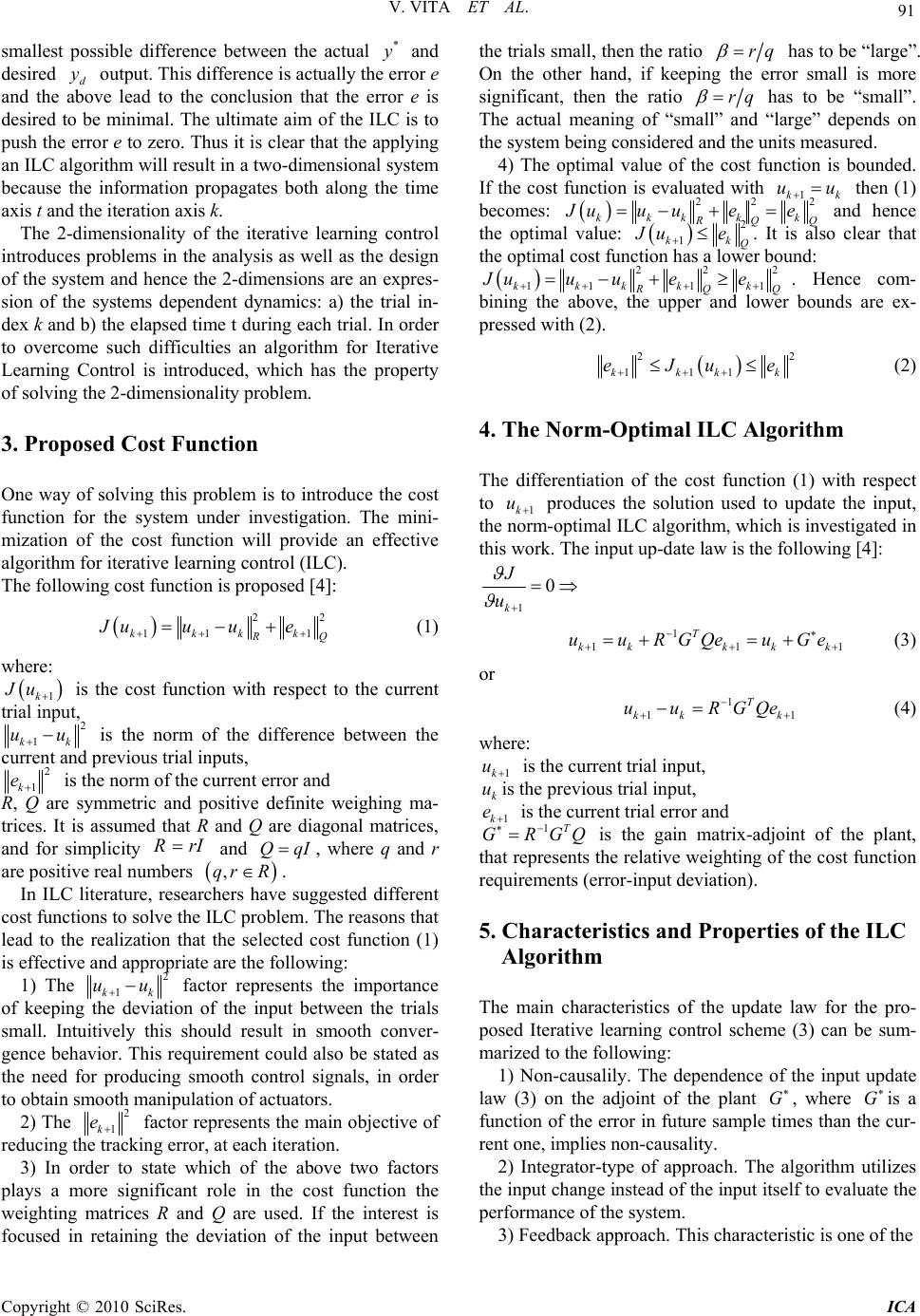 V. VITA ET AL. Copyright © 2010 SciRes. ICA 91 smallest possible difference between the actual * y and desired d y output. This difference is actually the error e and the above lead to the conclusion that the error e is desired to be minimal. The ultimate aim of the ILC is to push the error e to zero. Thus it is clear that the applying an ILC algorithm will result in a two-dimensional system because the information propagates both along the time axis t and the iteration axis k. The 2-dimensionality of the iterative learning control introduces problems in the analysis as well as the design of the system and hence the 2-dimensions are an expres- sion of the systems dependent dynamics: a) the trial in- dex k and b) the elapsed time t during each trial. In order to overcome such difficulties an algorithm for Iterative Learning Control is introduced, which has the property of solving the 2-dimensionality problem. 3. Proposed Cost Function One way of solving this problem is to introduce the cost function for the system under investigation. The mini- mization of the cost function will provide an effective algorithm for iterative learning control (ILC). The following cost function is proposed [4]: 22 11 1kkkk R Q Juu ue (1) where: 1k Ju is the cost function with respect to the current trial input, 2 1kk uu is the norm of the difference between the current and previous trial inputs, 2 1k e is the norm of the current error and R, Q are symmetric and positive definite weighing ma- trices. It is assumed that R and Q are diagonal matrices, and for simplicity r I R and QqI, where q and r are positive real numbers ,qr R. In ILC literature, researchers have suggested different cost functions to solve the ILC problem. The reasons that lead to the realization that the selected cost function (1) is effective and appropriate are the following: 1) The 2 1kk uu factor represents the importance of keeping the deviation of the input between the trials small. Intuitively this should result in smooth conver- gence behavior. This requirement could also be stated as the need for producing smooth control signals, in order to obtain smooth manipulation of actuators. 2) The 2 1k e factor represents the main objective of reducing the tracking error, at each iteration. 3) In order to state which of the above two factors plays a more significant role in the cost function the weighting matrices R and Q are used. If the interest is focused in retaining the deviation of the input between the trials small, then the ratio rq has to be “large”. On the other hand, if keeping the error small is more significant, then the ratio rq has to be “small”. The actual meaning of “small” and “large” depends on the system being considered and the units measured. 4) Τhe optimal value of the cost function is bounded. If the cost function is evaluated with 1kk uu then (1) becomes: 22 2 kkk kk R QQ J uuu ee and hence the optimal value: 2 1kk Q J ue . It is also clear that the optimal cost function has a lower bound: 22 2 111 1kkkk k R QQ Juu uee . Hence com- bining the above, the upper and lower bounds are ex- pressed with (2). 22 111kkkk eJue (2) 4. The Norm-Optimal ILC Algorithm The differentiation of the cost function (1) with respect to 1k u produces the solution used to update the input, the norm-optimal ILC algorithm, which is investigated in this work. The input up-date law is the following [4]: 1 0 k J u 1 111 T kkkk k uuRGQeuGe (3) or 1 11 T kk k uuRGQe (4) where: 1k u is the current trial input, k uis the previous trial input, 1k e is the current trial error and 1T GRGQ is the gain matrix-adjoint of the plant, that represents the relative weighting of the cost function requirements (error-input deviation). 5. Characteristics and Properties of the ILC Algorithm The main characteristics of the update law for the pro- posed Iterative learning control scheme (3) can be sum- marized to the following: 1) Non-causalily. The dependence of the input update law (3) on the adjoint of the plant G, where G is a function of the error in future sample times than the cur- rent one, implies non-causality. 2) Integrator-type of approach. The algorithm utilizes the input change instead of the input itself to evaluate the performance of the system. 3) Feedback approach. This characteristic is one of the 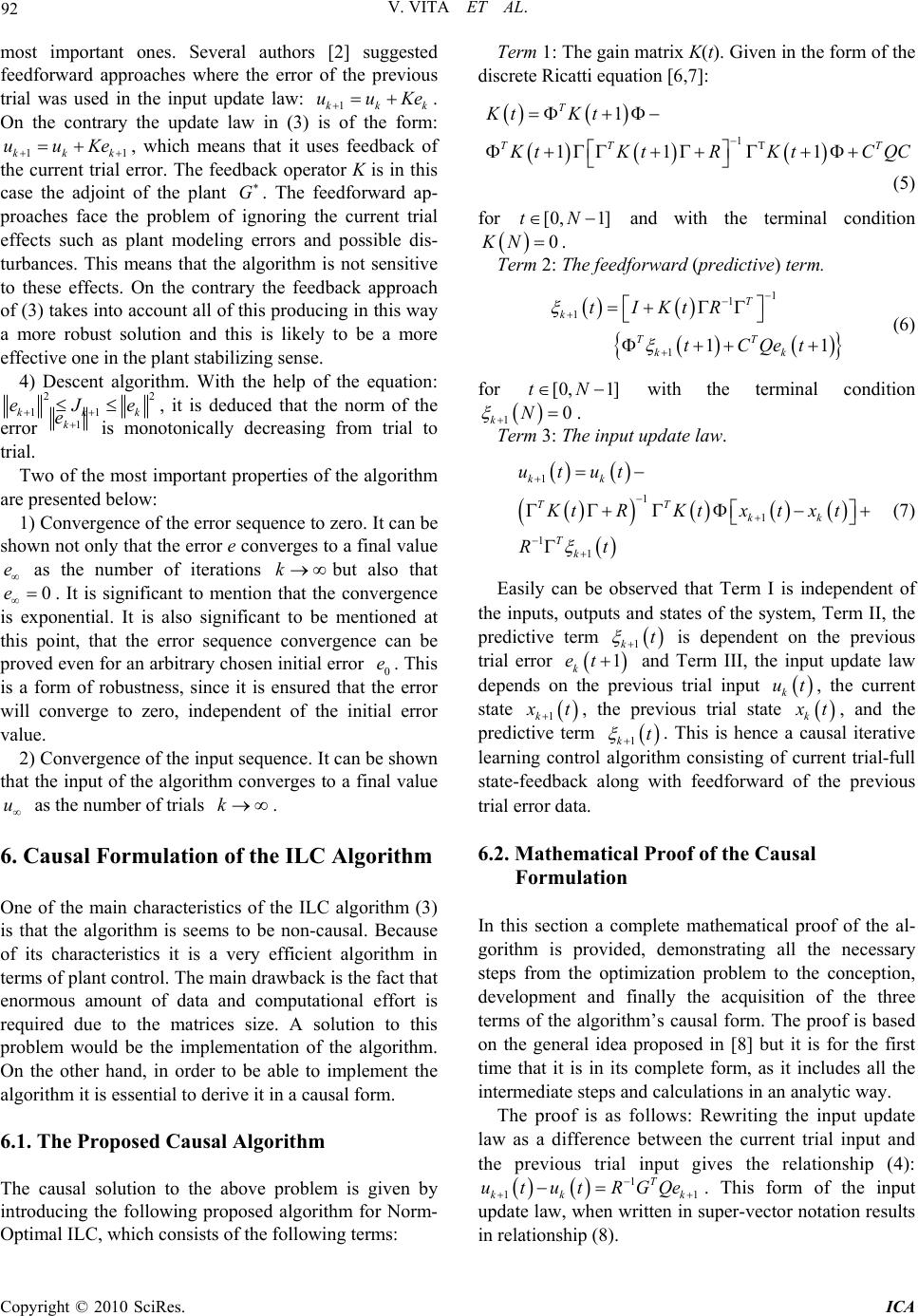 V. VITA ET AL. Copyright © 2010 SciRes. ICA 92 most important ones. Several authors [2] suggested feedforward approaches where the error of the previous trial was used in the input update law: 1kkk uuKe . On the contrary the update law in (3) is of the form: 11kkk uuKe , which means that it uses feedback of the current trial error. The feedback operator K is in this case the adjoint of the plant G. The feedforward ap- proaches face the problem of ignoring the current trial effects such as plant modeling errors and possible dis- turbances. This means that the algorithm is not sensitive to these effects. On the contrary the feedback approach of (3) takes into account all of this producing in this way a more robust solution and this is likely to be a more effective one in the plant stabilizing sense. 4) Descent algorithm. With the help of the equation: 22 11kkk eJe , it is deduced that the norm of the error 1k e is monotonically decreasing from trial to trial. Two of the most important properties of the algorithm are presented below: 1) Convergence of the error sequence to zero. It can be shown not only that the error e converges to a final value e as the number of iterations kbut also that 0e. It is significant to mention that the convergence is exponential. It is also significant to be mentioned at this point, that the error sequence convergence can be proved even for an arbitrary chosen initial error 0 e. This is a form of robustness, since it is ensured that the error will converge to zero, independent of the initial error value. 2) Convergence of the input sequence. It can be shown that the input of the algorithm converges to a final value u as the number of trials k. 6. Causal Formulation of the ILC Algorithm One of the main characteristics of the ILC algorithm (3) is that the algorithm is seems to be non-causal. Because of its characteristics it is a very efficient algorithm in terms of plant control. The main drawback is the fact that enormous amount of data and computational effort is required due to the matrices size. A solution to this problem would be the implementation of the algorithm. On the other hand, in order to be able to implement the algorithm it is essential to derive it in a causal form. 6.1. The Proposed Causal Algorithm The causal solution to the above problem is given by introducing the following proposed algorithm for Norm- Optimal ILC, which consists of the following terms: Term 1: The gain matrix K(t). Given in the form of the discrete Ricatti equation [6,7]: 1 1 11 1 T TT T Kt Kt K tKtRKtCQC (5) for [0, 1]tN and with the terminal condition 0KN . Term 2: The feedforward (predictive) term. 1 1 1 111 T k TT kk tIKtR tCQet (6) for [0, 1]tN with the terminal condition 10 kN . Term 3: The input update law. 1 1 1 1 1 kk TT kk T k utut KtRKtxtx t Rt (7) Easily can be observed that Term I is independent of the inputs, outputs and states of the system, Term II, the predictive term 1kt is dependent on the previous trial error 1 k et and Term III, the input update law depends on the previous trial input k ut, the current state 1k x t , the previous trial state k x t, and the predictive term 1kt . This is hence a causal iterative learning control algorithm consisting of current trial-full state-feedback along with feedforward of the previous trial error data. 6.2. Mathematical Proof of the Causal Formulation In this section a complete mathematical proof of the al- gorithm is provided, demonstrating all the necessary steps from the optimization problem to the conception, development and finally the acquisition of the three terms of the algorithm’s causal form. The proof is based on the general idea proposed in [8] but it is for the first time that it is in its complete form, as it includes all the intermediate steps and calculations in an analytic way. The proof is as follows: Rewriting the input update law as a difference between the current trial input and the previous trial input gives the relationship (4): 1 11 T kk k ututRGQe . This form of the input update law, when written in super-vector notation results in relationship (8).  V. VITA ET AL. Copyright © 2010 SciRes. ICA 93 21 1 1 2 1 1 13 1 1 1 1 00 1 11 2 0 22 3 00 11 00 0 N TTT TTTTTTTT kk k N TTT TTTTT kk k N kk k TTT TT kk k TT CC CC uu e uu e CC C RQuu e CC uN uNeN C (8) The difference of the control input 1kk ututu t at the tth sample (by examining the 1th t row of (8)) with 0tN , can be written: 1 1 1 1 Njt TT T kk jt utut RCQej (9) 1 1 1 1 Njt TTT kk jt ututR CQej (10) In order to derive a state space description of the ad- joint system, the discrete co-state pt is introduced, such that: 1 1 T kk ututRpt (11) Comparing (10) and (11) it follows that the co-state satisfies: 1 1 0 Njt TT jt ptCQe jtN (12) By expanding the sums in (12): 1 1 0 21 21 2 12 3 .... 12 3 .... 12 3.... Njt TT jt TT TT Nt TTT T TTT Nt TTT T TTT Nt TTT T ptCQe j ptCQet CQet CQet CQeN CQet CQet CQet CQeN CQet CQet CQet CQeN (13) but 2 12 3.... TTT Nt TT pt CQetCQet CQeN (14) Hence the above yields the recursion relation for pt: 110 TT ptCQetptt N (15) with 11 T pN CQet or equivalently 0pN . Consequently, the complete discrete input update law is as follows: 1 11 ,0 T kk k ututR pttN (16) 1 11 T kk k ututRpt (17) and 11 11 11,0 TT kk kk ptCQetpt pN (18) The main observation is the fact that the adjoint sys- tem has a terminal condition (at t = N) instead of an ini- tial condition; this is a sign of a non-causal solution. Equation (18) is an expression for the current trial co-state. Another expression for the co-state 1k pt can be calculated as follows: A standard technique [6,7] is to set the discrete co-state equal to: 1 1 1 11 k T kkk pt K tIRKtxt xtt (19) with a gain matrix K(t) and a correction term ξk+1(t). Both the terms K(t) and ξk+1(t) should be computed be- fore each trial. Lets set: 1 1T MtKtIRKt (20) and then substitute this into equation (19): 1 1 11 1 T kkk k ptKtIRKtxtx t t 111kkkk ptMt xtxtt (21) Setting the functions f(t) and g(t) as follows easily can be observed that these are independent of the states. 1 1 1 11 TT TT f tMtIKtRCQC IKtR Mt and 1 1 1 1 1 1 1 1 TT k TT kk gtI KtRt I KtRCQett 1) Calculating the (feedforward) predictive term 11 kt By setting g(t) = 0: 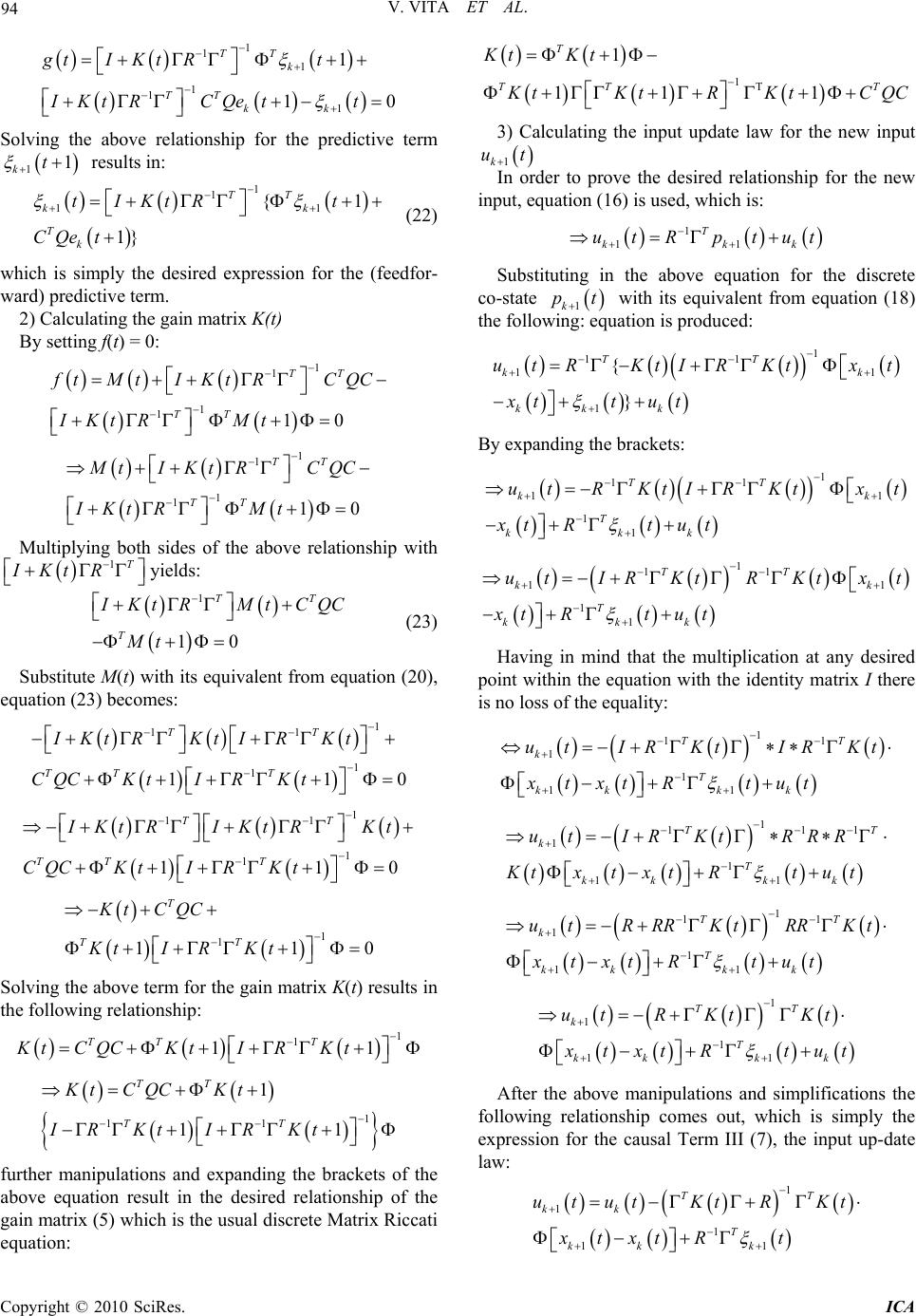 V. VITA ET AL. Copyright © 2010 SciRes. ICA 94 1 1 1 1 1 1 1 10 TT k TT kk gtI KtRt IKt RCQett Solving the above relationship for the predictive term 11 kt results in: 1 1 11 {1 1} TT kk T k tIKtR t CQe t (22) which is simply the desired expression for the (feedfor- ward) predictive term. 2) Calculating the gain matrix K(t) By setting f(t) = 0: 1 1 1 110 TT TT f tMtIKtRCQC IKt RMt 1 1 1 110 TT TT M tIKtRCQC IKtRMt Multiplying both sides of the above relationship with 1T IKtR yields: 1 10 TT T I Kt RMtCQC Mt (23) Substitute M(t) with its equivalent from equation (20), equation (23) becomes: 1 11 1 1 110 TT TT T I KtRKtIRKt CQCKtIRKt 1 11 1 1 110 TT TT T I Kt RIKt RKt CQCKtIRKt 1 1 110 T TT Kt CQC KtI RKt Solving the above term for the gain matrix K(t) results in the following relationship: 1 1 11 TT T Kt CQCKtIRKt 1 11 1 11 TT TT Kt CQCKt IR KtIR Kt further manipulations and expanding the brackets of the above equation result in the desired relationship of the gain matrix (5) which is the usual discrete Matrix Riccati equation: 1 1 11 1 T TT T Kt Kt K tKtRKtCQC 3) Calculating the input update law for the new input 1k ut In order to prove the desired relationship for the new input, equation (16) is used, which is: 1 11 T kkk utR ptut Substituting in the above equation for the discrete co-state 1k pt with its equivalent from equation (18) the following: equation is produced: 1 11 11 1 { } TT kk kk k utRKtIR Ktxt xttut By expanding the brackets: 1 11 11 1 1 TT kk T kkk utRKtIRKtxt xtRt ut 1 11 11 1 1 TT kk T kkk utIR KtR Ktxt xtRt ut Having in mind that the multiplication at any desired point within the equation with the identity matrix I there is no loss of the equality: 1 11 1 1 11 TT k T kk kk utIR KtIR Kt xtxt Rtut 1 111 1 1 11 TT k T kk kk utIR KtRRR Ktxtx tRtu t 1 11 1 1 11 TT k T kk kk utRRRKt RRKt xtxt Rtut 1 1 1 11 TT k T kk kk utR KtKt x txt Rtut After the above manipulations and simplifications the following relationship comes out, which is simply the expression for the causal Term III (7), the input up-date law: 1 1 1 11 TT kk T kk k ututKt RKt xtxt Rt  V. VITA ET AL. Copyright © 2010 SciRes. ICA 95 7. Conclusion In this paper an optimal iterative learning algorithm for discrete systems is analyzed. The algorithm’s properties and characteristics were presented with the most impor- tant feature to be that the error sequence converges to zero with an exponential rate for the case of discrete time plants. Finally, the complete causal formulation of the algorithm was derived in detail, consisting of optimal state feedback and optimal prediction feedforward. 8. References [1] Y. Chen and C. Wen, “Iterative Learning Control-Conver- Gence, Robustness and Applications,” Springer Verlag, London, 1999. [2] Z. Bien and J. X. Xu, “Iterative Learning Control-Analysis, Design, Integration and Applications,” Kluwer Academic Publishers, Dordrecht, 1998. [3] S. Arimoto, S. Kawamura and F. Miyazaki, “Bettering Operation of Dynamic Systems by Learning: A New Con- trol Theory for Servomechanism or Mechatronic Sys- tems,” Proceedings 23rd IEEE Conference on Decision and Control, Las Vegas, Nevada, 1984, pp. 1064-1069. [4] N. Amann, D. H. Owens and E. Roger, “Iterative Learning Control for Discrete Time Systems with Exponential Rate of Convergence,” IEE Proceeding of the Institution of Electrical Engineers on Control Theory and Applications, Vol. 143, No. 2, 1996, pp. 217-224. [5] K. L. Moore, “Iterative Learning Control for Deterministic Systems,” Advances in Industrial Control Series, Springer- Verlag, London, 1993. [6] K. J. Astrom and B. Wittenmark, “Computer controlled systems,” 2nd Edition, Prentice Hall, Englewoods Cliffs, 1990. [7] T. Kailath, “Linear Systems,” Prentice Hall, Englewoods Cliffs, 1980. [8] N. Amann, “Optimal Algorithms for Iterative Learning Control,” Ph.D. Dissertation, University of Exeter, UK, 1996. |

