Energy and Power Engineering, 2010, 2, 230-237
doi:10.4236/epe.2010.24034 Published Online November 2010 (http://www.SciRP.org/journal/epe)
Added Value of Power Control in Improving the
Integration of Wind Turbines in Weak Grid Conditions
Abdelaziz Arbaoui1, Mohamed Asbik2, Khalid Loudiyi3, Khalid Benhamou4
1ENSAM, Meknès Ismaïlia, Morocco
2Laboratoire de Physique des Matériaux et Modélisation des Systèmes (LP2MS), Unité associée au
CNRST-URAC: 08, Faculté des Sciences, Meknès, Maroc
3Al Akhawayn University, Ifrane, Morocco
4Sahara Wind Inc., Rabat, Morocco
Received May 13, 2010; revised July 7, 2010; accepted August 15, 2010
Abstract
For economical reasons, wind turbine systems must be located in favourable sites generating a higher pro-
ductivity. These are often located in areas with weak electric grid infrastructures. The constraints related to
this type of grids limit the penetration levels of wind energy. These constraints are mainly related to power
quality in the grid as well as the economical aspects of the project. In this study, we take into account the
slow voltage variations and the flicker phenomenon. The models used are based on the development of a set
of relations derived from engineering knowledge related to both technical and economical points of view.
The maximal penetration level of a fixed speed wind turbine system is determined for a given grid. The
power control has been investigated to improve wind turbine system integration. Obtained results show the
necessity to adapt technological choices to the requirements of weaker grids. Penetration levels and wind
turbine cost may be greatly improved using variable speed systems.
Keywords: Wind Turbine, Power Quality, Power Control, Weak Grid, Cost Modeling
1. Introduction
The current institutional and technical evolutions in the
field of electrical energy production schemes involve a
substantial growth of distributed generation using wind
turbine systems. Because of renewable and carbon-free
characteristics (cleanliness) of the energy produced, in-
corporating such systems has become a key element in the
new energy policies of many countries. Governments and
non-trading companies have shown an important interest
in achieving what can be considered as sustainable de-
velopment objectives through the extensive incorporation
of wind energy into electricity generation systems. Elec-
tricity distributors are interested in the viability and lower
costs as well as the quality of the energy produced. Aims
of investors have been focalized on potential profits
whereas designers, manufacturers and project managers
define the architecture of the system and its suitability to
the sites.
For economical reasons the wind turbine systems must
be implanted in more favourable windier sites which are
often located in areas with weak electric grid infrastruc-
tures. The constraints related to this type of grids limit
the penetration levels of wind energy. These constraints
are mainly those related to power quality in the connec-
tion node and to the economical aspects of the project.
The concept of power quality is related to the level of
satisfaction of the costumers, so the constraints related to
grid connection are imposed by the loads connected to it.
These constraints are described by norms that specify the
tolerances levels which must be guaranteed for the volt-
age as well as for the others disturbances usually met
within the grid. From a technical point of view, the power
quality constraints related to the weak grid that may limit
the penetration of wind energy depends on the character-
istics of both the wind turbine and the grid, they are
mainly [1,2]:
 Voltage variations: slow variations and fast varia-
tions known as flickers
 Harmonics and interharmonics,
 Stability and thermal capacity problems.
Several solutions exist to increase the penetration of the
wind energy production. These solutions use different

A. ARBAOUI ET AL. 231
technologies and concepts, and include the following:
 Grid reinforcement by installation of new lines;
 Control of reactive power;
 Introduction of load management;
 Dissipation of wind energy;
 Application of energy storage;
Each solution generates additional costs which can
impact the project’s profitability. As an example for grid
reinforcements, a line of 10 kV, 100 mm 2 Al PEX costs
30.000 $USA per miles [3].
In this paper we will take into account the slow voltage
variations and the flicker phenomenon constraints. The
objective is to study the value added of reactive power
control in improving the integration of wind turbines in
weak grid conditions. To reach this goal, the used models
are based on the development of a set of relations derived
from engineering knowledge related to both technical and
economical points of view. The technical knowledge base
describes the models of the grid and the wind turbine, the
interaction between them, and the power quality con-
straints. The economical knowledge base is related to the
electric energy production, project investment and wind
turbine components costs. All models are developed as a
Constraint Satisfaction Problem (CSP) which is then
implemented on a digital CSP solver based on interval
analysis to be solved [4].
2. Technical Knowledge Base
2.1. Weak Grid Model and Voltage Variations
Constraints
Various approaches are used to calculate the voltage
variation caused by the connection of a wind system:
determinist, temporal and probabilistic [5]. In this study
we use the first approach; the grid model used is repre-
sented in Figure 1. U1 is the voltage of infinite bus, U2
the voltage at the point of common coupling (PCC), and
Z is the equivalent impedance of the grid at this point.
The short-circuit power of the grid is given by:
22
11
22
Sc
UU
SZRX   (1)
When the voltage is constant, the short-circuit power is
constant if the impedance of the grid is constant. It should
nevertheless be specified that a given value of SSc can be
obtained for various values of the ratio X/R. This ratio
varies according to the level of the voltage, the configu-
Figure 1. Grid model.
ration of the grid, type of lines and their geometries.
The voltage variations are caused by variation of the
active power and the reactive power flow; the voltage at
the PPC can be expressed as Equation (2) [6]:
The authorized maximum voltage variation is defined
by the international commission of electrical engineering
(IEC 868). In Figure 2, the upper curve shows the
maximum permissible voltage variation with respect to
the frequency of the fluctuation [1]. For safety reasons,
the acceptable voltage variations defined by the lower
curve of the Figure 2 is adopted in this model.
Part (1) of the curve specifies that the slow voltage
variations are acceptable if they are lower than 3% of the
nominal voltage in the grid. For safety reasons we sup-
pose that the slow voltage variations are acceptable if they
are lower than 2.5% of the nominal voltage in grid.
12
1
(%) 1002.5
UU
UU

  (3)
Part (2) of the curve shows the acceptable limit of the
flicker phenomenon. This limit can be translated, ac-
cording to the frequency F, by the following constraint:
0.3
12
1
(%)1000.628
UU
UF
U


 (4)
Commonly, a point of the grid is considered weak if it
is poorly interconnected, far from the principal conven-
tional production units or if it is isolated. A current prac-
tice of the electrical engineers, is to evaluate the weakness
of a point of the grid by using the short-circuit power. The
value of this important parameter is provided by the dis-
tributor; it depends on the number and the characteristics
of the generation units feeding the grid as well as of the
equivalent impedance (lines and transformers impedances)
starting from the conventional production units up to the
point of study. According to the value of the short-circuit
power, the grid is considered weak or strong. The weaker
the grid is, the more it is affected by the disturbances
which come from the new built-in elements (loads or
distributed production systems). When the short-circuit
power is sufficiently high, it is considered that the quality
of electrical energy in the grid is not affected by new
   
2
22
2222
11
222
UU
URPXQ RPXQPQRX

 


(2)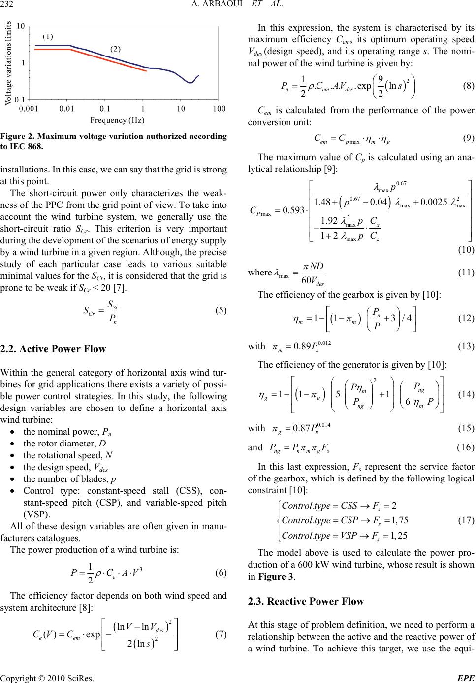

A. ARBAOUI ET AL. 232
Figure 2. Maximum voltage variation authorized according
to IEC 868.
installations. In this case, we can say that the grid is strong
at this point.
The short-circuit power only characterizes the weak-
ness of the PPC from the grid point of view. To take into
account the wind turbine system, we generally use the
short-circuit ratio SCr. This criterion is very important
during the development of the scenarios of energy supply
by a wind turbine in a given region. Although, the precise
study of each particular case leads to various suitable
minimal values for the SCr, it is considered that the grid is
prone to be weak if SCr < 20 [7].
Sc
Cr
n
S
SP  (5)
2.2. Active Power Flow
Within the general category of horizontal axis wind tur-
bines for grid applications there exists a variety of possi-
ble power control strategies. In this study, the following
design variables are chosen to define a horizontal axis
wind turbine:
 the nominal power, Pn
 the rotor diameter, D
 the rotational speed, N
 the design speed, Vdes
 the number of blades, p
 Control type: constant-speed stall (CSS), con-
stant-speed pitch (CSP), and variable-speed pitch
(VSP).
All of these design variables are often given in manu-
facturers catalogues.
The power production of a wind turbine is:
3
1
2e
PCAV   (6)
The efficiency factor depends on both wind speed and
system architecture [8]:


2
2
ln ln
() exp
2ln
des
eem
VV
CV C
s


  


(7)
In this expression, the system is characterised by its
maximum efficiency Cem, its optimum operating speed
Vdes (design speed), and its operating range s. The nomi-
nal power of the wind turbine is given by:

2
19
....exp ln
22
nemdes
PCAV s 



(8)
Cem is calculated from the performance of the power
conversion unit:
maxempm g
CC


 (9)
The maximum value of Cp is calculated using an ana-
lytical relationship [9]:

0.67
max
0.67 2
max max
max 2
max
max
1.480.04 0.0025
0.593
1.92
12
P
x
z
p
p
C
pC
pC








 













(10)
where max 60 des
ND
V


 (11)
The efficiency of the gearbox is given by [10]:

11 3/4
n
mm
P
P




 

 


 (12)
with 0.012 0.89
mn
P   (13)
The efficiency of the generator is given by [10]:

2
11 5 1 6
ng
m
gg
ng m
P
P
PP

 



 

 
 
 


 





(14)
with 0.014
0.87
gn
P   (15)
and ngn m gs
PP F



(16)
In this last expression, Fs represent the service factor
of the gearbox, which is defined by the following logical
constraint [10]:
.2
.1,75
.1,25
s
s
s
Control typeCSSF
Control typeCSPF
Control typeVSPF






(17)
The model above is used to calculate the power pro-
duction of a 600 kW wind turbine, whose result is shown
in Figure 3.
2.3. Reactive Power Flow
At this stage of problem definition, we need to perform a
relationship between the active and the reactive power of
a wind turbine. To achieve this target, we use the equi-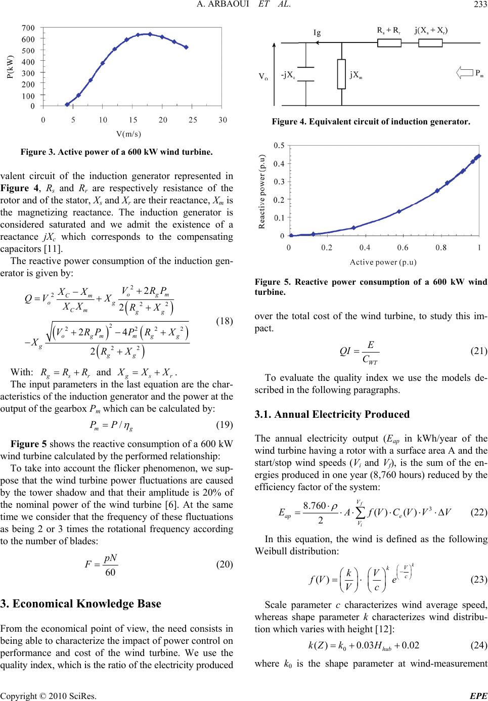

A. ARBAOUI ET AL. 233
Figure 3. Active power of a 600 kW wind turbine.
valent circuit of the induction generator represented in
Figure 4, Rs and Rr are respectively resistance of the
rotor and of the stator, Xs and Xr are their reactance, Xm is
the magnetizing reactance. The induction generator is
considered saturated and we admit the existence of a
reactance jXc which corresponds to the compensating
capacitors [11].
The reactive power consumption of the induction gen-
erator is given by:



2
2
22
2
2222
22
2
2
24
2
ogm
Cm
og
Cm gg
ogm mgg
g
gg
VRP
XX
QV X
XX RX
VRP PRX
XRX






(18)
With:
g
sr
RRR and
g
sr
X
XX.
The input parameters in the last equation are the char-
acteristics of the induction generator and the power at the
output of the gearbox Pm which can be calculated by:
/
mg
PP

 (19)
Figure 5 shows the reactive consumption of a 600 kW
wind turbine calculated by the performed relationship:
To take into account the flicker phenomenon, we sup-
pose that the wind turbine power fluctuations are caused
by the tower shadow and that their amplitude is 20% of
the nominal power of the wind turbine [6]. At the same
time we consider that the frequency of these fluctuations
as being 2 or 3 times the rotational frequency according
to the number of blades:
60
pN
F (20)
3. Economical Knowledge Base
From the economical point of view, the need consists in
being able to characterize the impact of power control on
performance and cost of the wind turbine. We use the
quality index, which is the ratio of the electricity produced
Figure 4. Equivalent circuit of induction generator.
Figure 5. Reactive power consumption of a 600 kW wind
turbine.
over the total cost of the wind turbine, to study this im-
pact.
WT
E
QI C  (21)
To evaluate the quality index we use the models de-
scribed in the following paragraphs.
3.1. Annual Electricity Produced
The annual electricity output (Eap in kWh/year of the
wind turbine having a rotor with a surface area A and the
start/stop wind speeds (Vi and Vf), is the sum of the en-
ergies produced in one year (8,760 hours) reduced by the
efficiency factor of the system:
3
8.760 () ()
2
f
i
V
ap e
V
EAfVCVVV
 

 
 (22)
In this equation, the wind is defined as the following
Weibull distribution:
()
k
V k
c
kV
fV e
Vc







 (23)
Scale parameter c characterizes wind average speed,
whereas shape parameter k characterizes wind distribu-
tion which varies with height [12]:
0
( )0.030.02
hub
kZ kH

 (24)
where k0 is the shape parameter at wind-measurement

A. ARBAOUI ET AL. 234
height Z0.
The vertical gradient of wind speed is considered by
introducing the following power law:
00
hub
H c
cZ




(25)
To have a quantitative assessment of the accuracy of
the estimated annual electricity described above, we refer
to the study done in 1998 by the Danish Energy Agency
[13]. This study is based on measured data in various
sites with respecting of the IEC standards procedures and
recommendations. In this reference, we founded the
power curves and the annual electricity production for
several standards wind turbines. To have a clear idea
about the exactitude of the used model, we have com-
pared the measured annual electricity production (Eref)
and that obtained by the used model for several standards
machines (E).
These comparisons demonstrate that the model calcu-
lations are in close agreement with a large quantity of
reference measured data. The Table 1 lists, for example,
the result of this comparison for NEG NTK 500/37 wind
turbine. According to this result, model calculations
closely fit measured annual electricity production when
the average wind speed is above 4 m/s. The difference
between the estimated and measured annual electricity
production is less than 3%. Since the sites, which are
economically viable, have an average wind speed greater
than 5 m/s, we can make out that the used model is quite
accurate to be used.
3.2. Wind Turbine Cost
The cost model of wind turbine encompasses aspects
related to the design and manufacture of such systems. It
Table 1. Comparison between the measured annual electri-
city produced by NEG NTK 500/37 wind turbine and that
obtained by the used model.
Average
wind speed
at hub High
Vm (m/s)
Weibull
Parameters
c k
(m/s)
E
(MWh/year)
Eref
(MWh/year)
Difference
(%)
4 4.51 2 202 225 −10.2
5 5.64 2 472 486 −2.9
6 6.77 2 818 816 0,25
7 7.90 2 1193 1176 1.45
8 9.03 2 1557 1532 1.6
9 10.16 2 1883 1858 1.4
10 11.28 2 2151 2138 0.6
is the sum of cost models of the components of the wind
turbine. A calibration factor FWT allows using real wind
turbine costs [14].
_, 1.1 WTWTcomponent iWT
i
CF CF 

(26)
The cost of some components is calculated from
weight models developed using engineering estimation
rules. These have been applied to the rotor, the transmis-
sion system, the nacelle, and the tower. As for the cost of
the generator and associated electrical equipment, it is
correlated with power rating. The models are not pre-
sented in this paper because they require a lot of pa-
rameters, but most of them can be found in reference
[10,15].
4. Value Added by Power Control
In this study, we have chosen the site characteristics
given in Table 2. To obtain a good judgement of total
field of the solutions, we introduced the variation domain
of the design variables gathered in Table 3. In our pre-
vious studies the global model is used to define a wind
turbine in adequacy with the wind in the site [16].
Figure 6 shows obtained results. These represent the
limit due to both slow voltage variation and flicker phe-
nomenon according to the X/R ratio. We notice the fol-
lowings:
 For the grids with a low X/R ratio, the short circuit
ratio is limited by the slow voltage variations.
 For the grids having a large X/R ratio, the short
circuit ratio is limited by the flicker phenomenon.
This is explained by the fact that, grids with low X/R
ratio have their active power flow causing the slow volt-
Table 2. Characteristics of the investigated site.
Table 3. Design variables and their domain of variation.
k0 c
0
 Z0 U
1 S Sc
1.2 8 0.12 30 11 kV 10 MVA
Design variable Domain of variation
D (m) [20,80] with a step of 10 m
Pn (kW) [400,2000] with a step of 25 kW
Vdes (m/s) [6,12] with a step of 2 m/s
Hhub (m) [35,70] with a step of 10 m
N (tr/mn) [15,50] with a step of 5 tr/mn
Control type «PVC» or «SVC» or «PVV»
p 2 or 3

A. ARBAOUI ET AL. 235
Figure 6. Minimum short-circuit ratio for the constant speed
system.
age variation. However grids with high X/R ratio have
their reactive power flow as the main cause for the slow
voltage variation [17].
For the slow variation constraint, Figure 7 represents
the minimum short circuit ratio for a variable speed
compared with a constant speed system. In order to high-
light the importance of the reactive power control, we
consider here that cos 1

 for the variable speed sys-
tem.
We point out that the reactive power control makes it
possible to increase the penetration of wind energy when
the X/R ratio is higher than 2.7. In the case where X/R
ratio lowers than 2.7, when the rectifier is with forced
commutation, it is possible to control judiciously the
cos

in order to obtain a penetration level equal or
higher than what’s achieved with the constant speed sys-
tem [6]. Figure 8 shows that the use of a variable speed
control makes it possible to attenuate the flicker phe-
nomenon. Contrary to the result obtained for the constant
speed system, the fact of having cos 1

 implies that
the flicker phenomenon is not any more one criterion of
a grid evaluation.
The results above show the positive impact of power
control on the maximal penetration level which repre-
sents the technical added value of this concept. To have a
good idea on this impact, for an X/R = 4 we can install a
1425 kW variable speed wind turbine against only 500
kW if the system is a constant speed one.
The power control has also a positive impact on the
quality index of the wind turbine as shown by the results
obtained from the use of economical knowledge base in
Table 3 and Figure 9.
The increase in the quality index is due to the reduc-
tion in the cost of the system. The annual energy pro-
duced is the same for the two concepts. In fact, the en-
ergy model used doesn’t take into account the influence
of the control type as Equation (17) lets us believe by
introducing the service factor of the gearbox Fs. This last
Figure 7. Minimum short-circuit ratio for slow variation con-
straint: Comparison between the constant and variable speed
systems.
Figure 8. Minimum short-circuit ratio for variable speed
system.
Figure 9. Cost reduction for the variable speed system.
Table 4. Criteria comparison for a 1425kW wind turbine.
Criteria
Wind turbines
IQ E CWT
Variable speed 4.7 3.1 0.6
Constant speed 4.18 3.1 0.74
factor has however a great influence on the components
costs of wind turbine (for more details, see references
[10,15]). By using a variable speed control a decrease in
the rotor cost becomes realistic; but the greatest part of
this reduction is offered by the gearbox. The gain which

A. ARBAOUI ET AL. 236
must be carried out at the level of these tow components
will certainly compensates for the 40% increase in the
electrical unit, while the gain at the level of the nacelle is
insignificant.
5. Conclusions
In this work illustrates the added value of power control in
improving the integration of wind turbines in weak grid
conditions. We took into account wind turbines connec-
tion to the weak grid through slow voltage variations and
Flicker phenomenon constraints. Ours models are based
on the development of a set of relations derived from
engineering knowledge related to both technical and
economical points of view.
The technical knowledge base determines the maxi-
mum penetration level of fixed-speed wind turbine sys-
tems in a given grid, and evaluates the impact of reactive
power control on the penetration level. The impact of
reactive power control on wind turbine components costs
was studied through the economical knowledge base.
All models were developed as a Constraint Satisfac-
tion Problem (CSP) which is then implemented on a
digital CSP solver based on interval analysis to be solved.
Obtained results show the necessity to adapt technologi-
cal choices to the requirements of weaker grids. Penetra-
tion levels and wind turbine cost may be greatly im-
proved using variable speed systems.
For future research investigations, it would be inter-
esting to integrate the influence of power control on the
efficiency and effectiveness of a wind turbine. This may
provide us a good judgement about the genuine added
value of the economic point of view.
6. References
[1] J. O. G Tande, “Applying Power Quality Characteristics
off Wind Turbines for Assessing Impact one Voltage
Quality,” Wind Energy, Vol. 5, No. 1, 2002, pp. 37-52.
[2] P. Bousseau, et al., “Solutions for the Grid Integration of
Wind Farms—A Survey”, Wind Energy, Vol. 9, No. 1,
2006, pp. 13-25.
[3] J. O. G Tande, “Exploitation of Wind-Energy Resources
in Proximity to Weak Electric Grids,” Applied Energy,
Vol. 65, No. 1, 2000, pp. 395-401.
[4] A. Arbaoui and M. Asbik, “Constraints Based Decision
Support for Site-Specific Preliminary Design of Wind
Turbines,” Energy and Power Engineering, Vol. 2, No. 3,
2010, pp. 161-170.
[5] N. G. Boulaxis, S. A. Papathanassiou and M. P. Papado-
poulos, “Wind Turbine Effect on the Voltage Profile of
Distribution Networks,” Renewable Energy, Vol. 25, No. 3,
2002, pp. 401-415.
[6] A. Larson, “The Power Quality of Wind Turbines” Ph.D.
Thesis for Chalmers University of Technology, Sweden,
2000.
[7] O. Alejandro, “Issues Regarding the Integration of Induc-
tion Wind Turbines in Weak Electrical Networks,” Nor-
dic Wind Power Conference, Gothenburg, 2004.
[8] C. T. Kiranoudis, N. G. Voros and Z. B. Maroulis,
“Short-Cut Design of Wind Farms,” Energy Policy, Vol.
29, No. 7, 2001, pp. 567-578.
[9] A. Spera, “Wind Turbine Technology,” The American
Society of Mechanical Engineering, 1998.
[10] R. Harrison and G. Jenkins, “Cost Modelling of Horizon-
tal Axis Wind Turbines (Phase 2),” ETSU W/34/00170/
REP, University of Sunderland, 1994.
[11] A. E. Feijoo, “Infuencia de los Parques Eolicos en la
Seguridad Estacionaria y Calidad del Onda de Redes
Eléctricas de Gran Dimension,” PhD Thesis of Vigo
University, Vigo, 1998.
[12] I. Troen and E. L. Petersen, “European Wind Atlas,” Riso
National Laboratory, Roskilde, 1989.
[13] H. Petersen, “Comparison of Wind Turbines Based on
Power Curve Analysis,” Report Made for Danish Energy
Agency’s, 1998.
[14] T. Diveux, P. Sebastian, D. Bernard, J. R. Puiggali and J.
Y. Grandidier, “Horizontal Axis Wind Turbine Systems:
Optimization Using Genetic Algorithms,” Wind Energy,
Vol. 4, No. 4, 2001, pp. 151-171.
[15] A. Arbaoui, “Aide à la Décision Pour la Définition d’un
Système Eolien, Adéquation au Site et à un Réseau
Faible,” Ph.D Thesis of the Ecole Nationale Supérieure
d’Arts et Métiers, Bordeaux, 2006.
[16] A. Arbaoui, J. P. Nadeau and P. Sébastian, “Adéquation
Site et Système Eolien Eléments d’aide à la Décision par
la Modélisation par Contraintes,” Revue des Energies
Renouvelables, Vol. 8, No. 2, 2005, pp. 81-94.
[17] T. Ackermann, et al., “Embedded Wind Generation in
Weak Grids-Economic Optimisation and Power Quality
Simulation,” Renewable Energy, Vol. 18, No. 2, 1999, pp.
205-221.

A. ARBAOUI ET AL. 237
Notation
A rotor swept area (m2),
C Weibull distribution scale parameter (m/s)
Ccomponent cost of component
Ce: system efficiency factor
Cem maximum system efficiency factor
CP rotor power coefficient
Cpmax maximum power coefficient
CX blade profile drag coefficient
CZ blade profile lift coefficient
CWT total cost of wind turbine (MEuros)
D rotor diameter (m)
E annual electricity produced (GWh/year)
Fs service factor of gearbox
FWT cost calibration factor
F Weibull distribution probability density
Hhub hub height (m)
K Weibull distribution shape parameter
N rotor rotation speed (rev/min)
P blade number
Pn nominal power (kW)
Png generator power rating (kW)
QI quality index
Rr rotor resistance of the induction generator (Ω)
Rs stator resistance of the induction generator (Ω)
S operating range
V0 voltage out put of the induction generator
V wind speed (m/s)
Vdes design wind speed (m/s)
Vf network-disconnection speed (m/s)
Vi network-connection speed (m/s)
Vm average wind speed at hub height (m/s)
Vtip blade tip speed (m/s)
Xm magnetizing reactance (Ω)
Xc compensating capacitors reactance (Ω)
Greek
 wind shear factor
max maximum tip speed ratio
 air density (kg/m3)
m gearbox efficiency
g generator efficiency
g generator efficiency factor
m gearbox efficiency factor