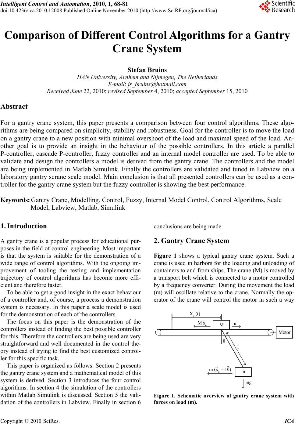Intelligent Control and Automation, 2010, 1, 68-81
doi:10.4236/ica.2010.12008 Published Online November 2010 (http://www.SciRP.org/journal/ica)
Comparison of Different Control Algorithms for a Gantry
Crane System
Stefan Bruins
HAN University, Ar nhem and Nijmegen, The Netherlands
Received June 22, 2010; revised September 4, 2010; accepted September 15, 2010
Abstract
For a gantry crane system, this paper presents a comparison between four control algorithms. These algo-
rithms are being compared on simplicity, stability and robustness. Goal for the controller is to move the load
on a gantry crane to a new position with minimal overshoot of the load and maximal speed of the load. An-
other goal is to provide an insight in the behaviour of the possible controllers. In this article a parallel
P-controller, cascade P-controller, fuzzy controller and an internal model controller are used. To be able to
validate and design the controllers a model is derived from the gantry crane. The controllers and the model
are being implemented in Matlab Simulink. Finally the controllers are validated and tuned in Labview on a
laboratory gantry scrane scale model. Main conclusion is that all presented controllers can be used as a con-
troller for the gantry crane system but the fuzzy controller is showing the best performance.
Keywords: Gantry Crane, Modelling, Control, Fuzzy, Internal Model Control, Control Algorithms, Scale
Model, Labview, Matlab, Simulink
1. Introduction
A gantry crane is a popular process for educational pur-
poses in the field of control engineering. Most important
is that the system is suitable for the demonstration of a
wide range of control algorithms. With the ongoing im-
provement of tooling the testing and implementation
trajectory of control algorithms has become more effi-
cient and therefore faster.
To be able to get a good insight in the exact behaviour
of a controller and, of course, a process a demonstration
system is necessary. In this paper a scale model is used
for the demonstration of each of the controllers.
The focus on this paper is the demonstration of the
controllers instead of finding the best possible controller
for this. Therefore the controllers are being used are very
straightforward and well documented in the control the-
ory instead of trying to find the best customized control-
ler for this specific task.
This paper is organized as follows. Section 2 presents
the gantry crane system and a mathematical model of this
system is derived. Section 3 introduces the four control
algorithms. In section 4 the simulation of the controllers
within Matlab Simulink is discussed. Section 5 the vali-
dation of the controllers in Labview. Finally in section 6
conclusions are being made.
2. Gantry Crane System
Figure 1 shows a typical gantry crane system. Such a
crane is used in harbors for the loading and unloading of
containers to and from ships. The crane (M) is moved by
a transport belt which is connected to a motor controlled
by a frequency converter. During the movement the load
(m) will oscillate relative to the crane. Normally the op-
erator of the crane will control the motor in such a way
Figure 1. Schematic overview of gantry crane system with
forces on load (m).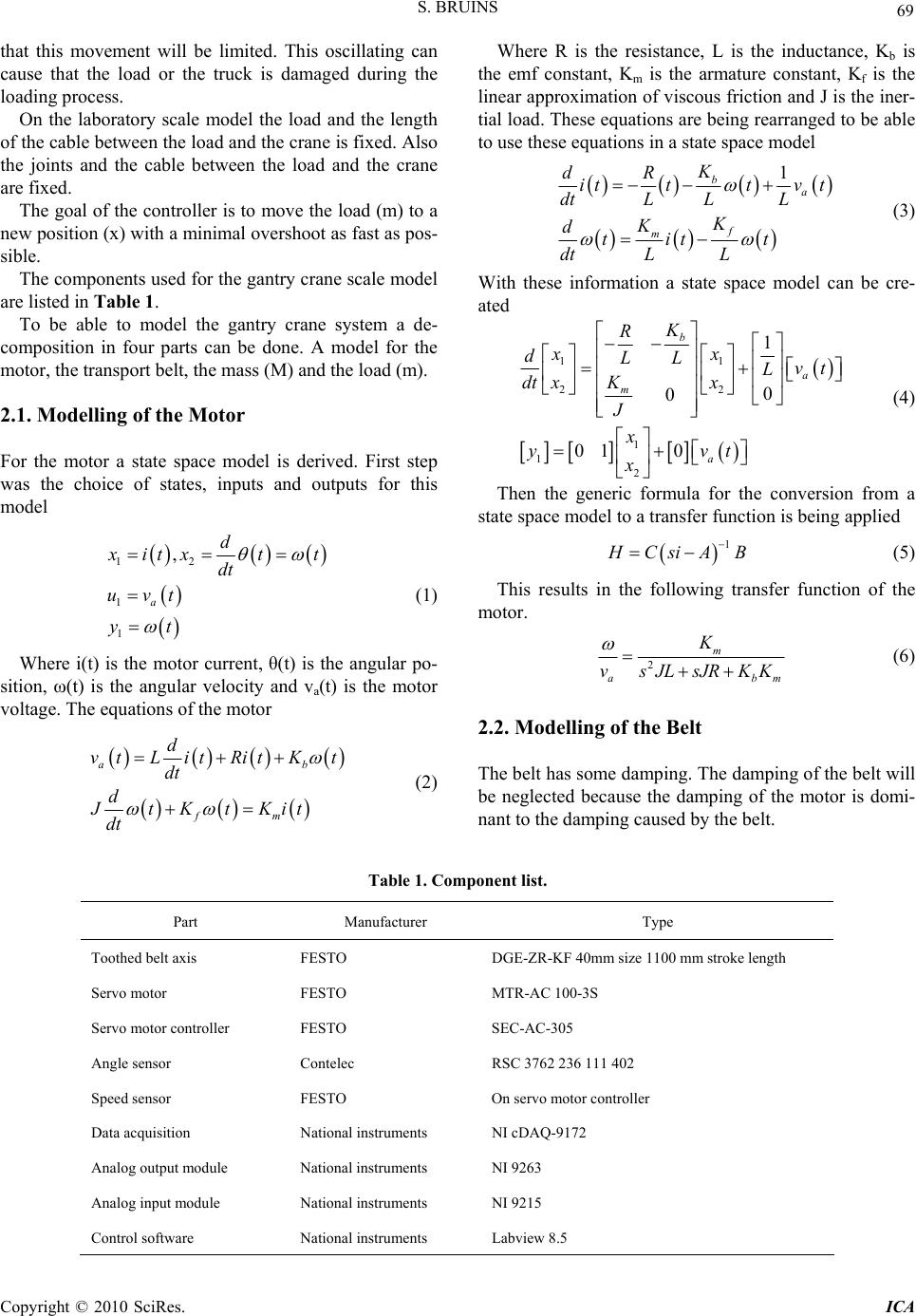

S. BRUINS
69
that this movement will be limited. This oscillating can
cause that the load or the truck is damaged during the
loading process.
On the laboratory scale model the load and the length
of the cable between the load and the crane is fixed. Also
the joints and the cable between the load and the crane
are fixed.
The goal of the controller is to move the load (m) to a
new position (x) with a minimal overshoot as fast as pos-
sible.
The components used for the gantry crane scale model
are listed in Table 1.
To be able to model the gantry crane system a de-
composition in four parts can be done. A model for the
motor, the transport belt, the mass (M) and the load (m).
2.1. Modelling of the Motor
For the motor a state space model is derived. First step
was the choice of states, inputs and outputs for this
model
  


12
1
1
,
a
d
x
it xtt
dt
uvt
yt





(1)
Where i(t) is the motor current, θ(t) is the angular po-
sition, ω(t) is the angular velocity and va(t) is the motor
voltage. The equations of the motor
 
 
ab
fm
d
vtL itRitKt
dt
d
JtKtKit
dt




(2)
Where R is the resistance, L is the inductance, Kb is
the emf constant, Km is the armature constant, Kf is the
linear approximation of viscous friction and J is the iner-
tial load. These equations are being rearranged to be able
to use these equations in a state space model
 
 
1
ba
f
m
K
dR
itttv t
dtL LL
K
K dtit t
dtL L


 

(3)
With these information a state space model can be cre-
ated

  
11
22
1
1
2
1
0
0
01 0
b
a
m
a
K R
xx
dLL vt
L
xx K dt
J
x
yvt
x

 

 
 
 

  




 

(4)
Then the generic formula for the conversion from a
state space model to a transfer function is being applied

1
H
Csi AB

 (5)
This results in the following transfer function of the
motor.
2
m
abm
K
v
s
JLsJRK K

 (6)
2.2. Modelling of the Belt
The belt has some damping. The damping of the belt will
be neglected because the damping of the motor is domi-
nant to the damping caused by the belt.
Table 1. Component list.
Part Manufacturer Type
Toothed belt axis FESTO DGE-ZR-KF 40mm size 1100 mm stroke length
Servo motor FESTO MTR-AC 100-3S
Servo motor controller FESTO SEC-AC-305
Angle sensor Contelec RSC 3762 236 111 402
Speed sensor FESTO On servo motor controller
Data acquisition National instruments NI cDAQ-9172
Analog output module National instruments NI 9263
Analog input module National instruments NI 9215
Control software National instruments Labview 8.5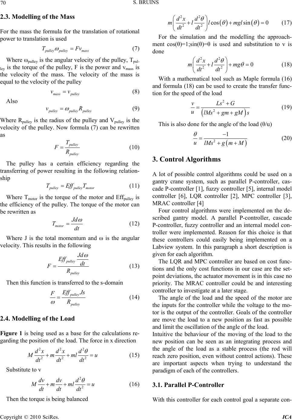

S. BRUINS
70
2.3. Modelling of the Mass
For the mass the formula for the translation of rotational
power to translation is used
p
ulley pulleymass
TFv

 (7)
Where ωpulley is the angular velocity of the pulley, Tpul-
ley is the torque of the pulley, F is the power and vmass is
the velocity of the mass. The velocity of the mass is
equal to the velocity of the pulley
mass pulley
vv (8)
Also
p
ulleypulley pulley
vR

 (9)
Where Rpulley is the radius of the pulley and Vpulley is the
velocity of the pulley. Now formula (7) can be rewritten
as
p
ulley
p
ulley
T
FR  (10)
The pulley has a certain efficiency regarding the
transferring of power resulting in the following relation-
ship
p
ulleypulley motor
TEffT (11)
Where Tmotor is the torque of the motor and Effpulley is
the efficiency of the pulley. The torque of the motor can
be rewritten as
motor
J
d
Tdt

 (12)
Where J is the total momentum and ω is the angular
velocity. This results in the following
pulley
pulley
J
d
Eff dt
FR

 (13)
Then this function is transferred to the s-domain
pulley
pulley
Eff Js
F
R

 (14)
2.4. Modelling of the Load
Figure 1 is being used as a base for the calculations re-
garding the position of the load. The force in x direction
22 2
22 2
dx dxd
M
mml u
dt dtdt

 
(15)
Substitute to v
2
2
dv dvd
M
mml u
dt dtdt

  (16)
Then the torque is being balanced
 
22
22
cossin 0
dx d
ml lmgl
dt dt





 (17)
For the simulation and the modelling the approach-
ment cos(θ)=1;sin(θ)=θ is used and substitution to v is
done
22
22 0
dx d
mlmg
dt dt






(18)
With a mathematical tool such as Maple formula (16)
and formula (18) can be used to create the transfer func-
tion for the speed of the load

2
2
vLsG
ulMsgmgM s

 (19)
This is also done for the angle of the load (θ/u)

2
1
ulMsg mM
 
 (20)
3. Control Algorithms
A lot of possible control algorithms could be used on a
gantry crane system, such as parallel P-controller, cas-
cade P-controller [1], fuzzy controller [5], internal model
controller [6], LQR controller [2], MPC controller [3],
MRAC controller [4]
Four control algorithms were implemented on the de-
scribed gantry model. A parallel P-controller, cascade
P-controller, fuzzy controller and an internal model con-
troller were implemented. Reason for this choice is that
these controllers could easily being implemented on a
Labview system. In this paragraph a short description is
given for each algorithm.
The LQR and MPC controller are based on cost func-
tions and the only cost functions in our case are the set-
point deviations, the actuator movement is in this case no
priority. The MRAC controller could be and interesting
controller to investigate at a later stage.
The angle of the load and the speed of the motor are
the inputs for the controller while the voltage to the mo-
tor is the output of the controller. Goals of the controller
are move the load to a new position as fast as possible
and limit the oscillation of the angle of the load.
Intuitive the behaviour of the moving of the load to the
new position can be seen as an integrating process and
the angle of the load as a stable process (the rod will
reach zero position, even without control actions). These
are important aspects when trying to understand the
paradigm of each of the controllers.
3.1. Parallel P-Controller
With this controller for each control goal a separate con-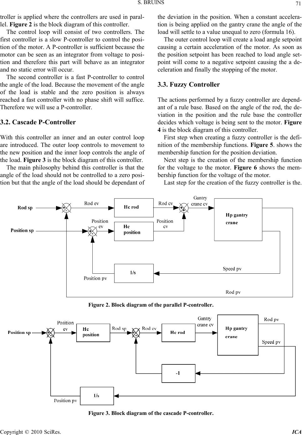

S. BRUINS
71
troller is applied where the controllers are used in paral-
lel. Figure 2 is the block diagram of this controller.
The control loop will consist of two controllers. The
first controller is a slow P-controller to control the posi-
tion of the motor. A P-controller is sufficient because the
motor can be seen as an integrator from voltage to posi-
tion and therefore this part will behave as an integrator
and no static error will occur.
The second controller is a fast P-controller to control
the angle of the load. Because the movement of the angle
of the load is stable and the zero position is always
reached a fast controller with no phase shift will suffice.
Therefore we will use a P-controller.
3.2. Cascade P-Controller
With this controller an inner and an outer control loop
are introduced. The outer loop controls to movement to
the new position and the inner loop controls the angle of
the load. Figure 3 is the block diagram of this controller.
The main philosophy behind this controller is that the
angle of the load should not be controlled to a zero posi-
tion but that the angle of the load should be dependant of
the deviation in the position. When a constant accelera-
tion is being applied on the gantry crane the angle of the
load will settle to a value unequal to zero (formula 16).
The outer control loop will create a load angle setpoint
causing a certain acceleration of the motor. As soon as
the position setpoint has been reached to load angle set-
point will come to a negative setpoint causing the a de-
celeration and finally the stopping of the motor.
3.3. Fuzzy Controller
The actions performed by a fuzzy controller are depend-
ant of a rule base. Based on the angle of the rod, the de-
viation in the position and the rule base the controller
decides which voltage is being sent to the motor. Figure
4 is the block diagram of this controller.
First step when creating a fuzzy controller is the defi-
nition of the membership functions. Figure 5 . shows the
membership function for the position deviation.
Next step is the creation of the membership function
for the voltage to the motor. Figure 6 shows the mem-
bership function for the voltage of the motor.
Last step for the creation of the fuzzy controller is the.
Figure 2. Block diagram of the parallel P-controller.
Figure 3. Block diagram of the c ascade P-contr o l ler.

S. BRUINS
72
Figure 4. Block diagram of the fuz zy controller .
Figure 5. Membership function position deviation and load
angle deviation.
Figure 6. Membership function motor CV.
rulebase which determines how the input membership
functions are related to the output membership functions
Table 2. displays the used rule base.
The rulebase can be read as follow. If the load angle
deviation is left and the position deviation is center the
motor CV will be right. Figure 7 gives a graphical rep-
resentation of the behaviour of the fuzzy controller.
To make the system more flexible gains are connected
to the fuzzy controller inputs and outputs (K rod, K pos
and Kcv). With these gains the normalized membership
functions can be stretched or compressed without
changing the membership functions.
3.4. Internal Model Controller
The internal model controller shows the same behaviour
as the parallel P-controller. The only difference is that
the control actions are being performed on a digital
Table 2. Rulebase fuzzy controller.
Position deviation
Left Center Right
Left Left Right Upper right
Center Left Center Right
Load angle
deviation
Right Upper left Left Right
Figure 7. Fuzzy contro lle r input-output r e l ationships.
model instead of the process. The control signals are
being based on the predicted behaviour of the process.
Differences between the model and the process are fed
back with a low pass filter. This type of controller is very
suitable in cases where the sensors suffer from noise.
Figure 8 is the block diagram of this controller.
3.4.1. Discrete Motor Model
Equation (6) is transferred to the z-domain by applying
the following function
1z
sTz

 (21)

S. BRUINS
73
Figure 8. Block diagram of the internal model controller.
Where T is the sample rate. This results in the follow-
ing discrete transfer function
22
2222
2
m
bm
KTz
J
LzJLzJLJRTzJRTzK KTz  (22)
This is equal to x/u resulting in the following rela-
tionship
22
22 22
2
bm m
x
JLzxJLzxJL xJRTzxJRTz
xKKTz uKTz
 
 (23)
After some simplification and adaptation for imple-
mentation the relationship between input and output can
be rewritten as

212
2
2
m
bm
uK TLJJRTxzLJxz
xLJJRTK KT

 
 (24)
3.4.2. Discrete Mass Model
The model of the mass as in formula (15) has a differen-
tial action. To simplify the digital model the differential
action is shifted to the discrete movement model and the
discrete load model. In this way the model shows no dy-
namics and therefore can directly being applied in the
discrete domain.
pulley
pulley
FEff J
sR

 (25)
3.4.3. Discrete movement model
Next part to be transferred to the discrete time domain is
the transfer function of the movement of the motor. A
transfer function for a static load has to be created. For-
mula (16) is used without the movement of the load
dv dv
M
mu
dt dt

 (26)
Then this function is transferred to the s-domain


M
msv u

 (27)
Resulting in the following transfer function

1v
uMms
 (28)
Taken into account that the result of the discrete mass
model as described in formula (25) is the integral of u,
the transfer function can be rewritten as

1x
uMms
 (29)
Formula (21) is applied on this transfer function to
transfer it to the z-domain resulting in the following dis-
crete transfer function

1
xTz
uMmz


 (30)
This is equal to x/u resulting in the following rela-
tionship




1
x
mM zuTz
(31)
After some simplification and adaptation for imple-
mentation the relationship between input and output can
be rewritten as


1
uTmMxz
xmM


 (32)
3.4.4. Discrete Load Model
Next part to be transferred to the discrete time domain is

S. BRUINS
74
the transfer function of the angle of the load. Taken into
account that the result of the discrete mass model is the
integral of u, the transfer function as in formula (20) can
be rewritten as

2
s
lMsg mM
 (33)
Formula (21) is applied on this transfer function to
transfer it to the z-domain resulting in the following dis-
crete transfer function


222
1
2
Tz z
lMzlMzlMg mM T z

 (34)
This is equal to x/u resulting in the following rela-
tionship




222
21xlMzlMz lMgmMTzuTzz 
(35)
After some simplification and adaptation for imple-
mentation the relationship between input and output can
be rewritten as

112
2
2uT uTzxlMzxlMz
xlMg mM T

 
 (36)
3.4.5. Total Discrete Model
The total digital model is the result of the block diagram
of formulas as displayed in Figure 9.
4. Simulation
The control algorithms were tested in Matlab Simulink.
Figure 10 shows the setup for the simulation of the gan-
try crane.
Table 3 shows the parameter list used for the simula-
tion.
Figure 11 shows the result when applying a step of
0.2 V on the Gantry crane.
Next the controllers are simulated. Table 4, 5, 6 and 7
shows the parameter list with controller settings
Figure 12 shows the result when a step of 0.4 is ap-
plied on the position SP for all the controllers.
The performance for all the controllers are shown in
Table 8.
When comparing the simulated controllers the similar-
ity between the parallel P-controller and the cascade
P-controller is obvious. The performance and the step
response are almost the same.
The fuzzy controller is showing the best performance.
This is mainly caused by the fact that the Gantry Crane
CV is limited by the output membership function of the
fuzzy controller. At the other controllers only the satura-
tion of the actuators are limiting the Gantry Crane CV.
Limiting is important because a large dCV/dt will cause
large oscillations on the rod angle.
The internal model controller is showing the worst
performance, although the differences are small. Impor-
tant factor is that the time constant of the rod angle filter
is larger then the time constant of the rod angle. There-
fore the controller is not able to correct the differences
between model and process fast enough. When reducing
the time constant of the filter the influence of the model
will be reduced and the system will be more vulnerable
for noise. Figure 13 show the difference between the
simulated process and the digital model.
Figure 9. Gantry crane digital model overview.
Figure 10. Gantry crane model overview.

S. BRUINS
75
Figure 11. Gantry crane step response.
Figure 12. Gantry crane simulated controllers step response.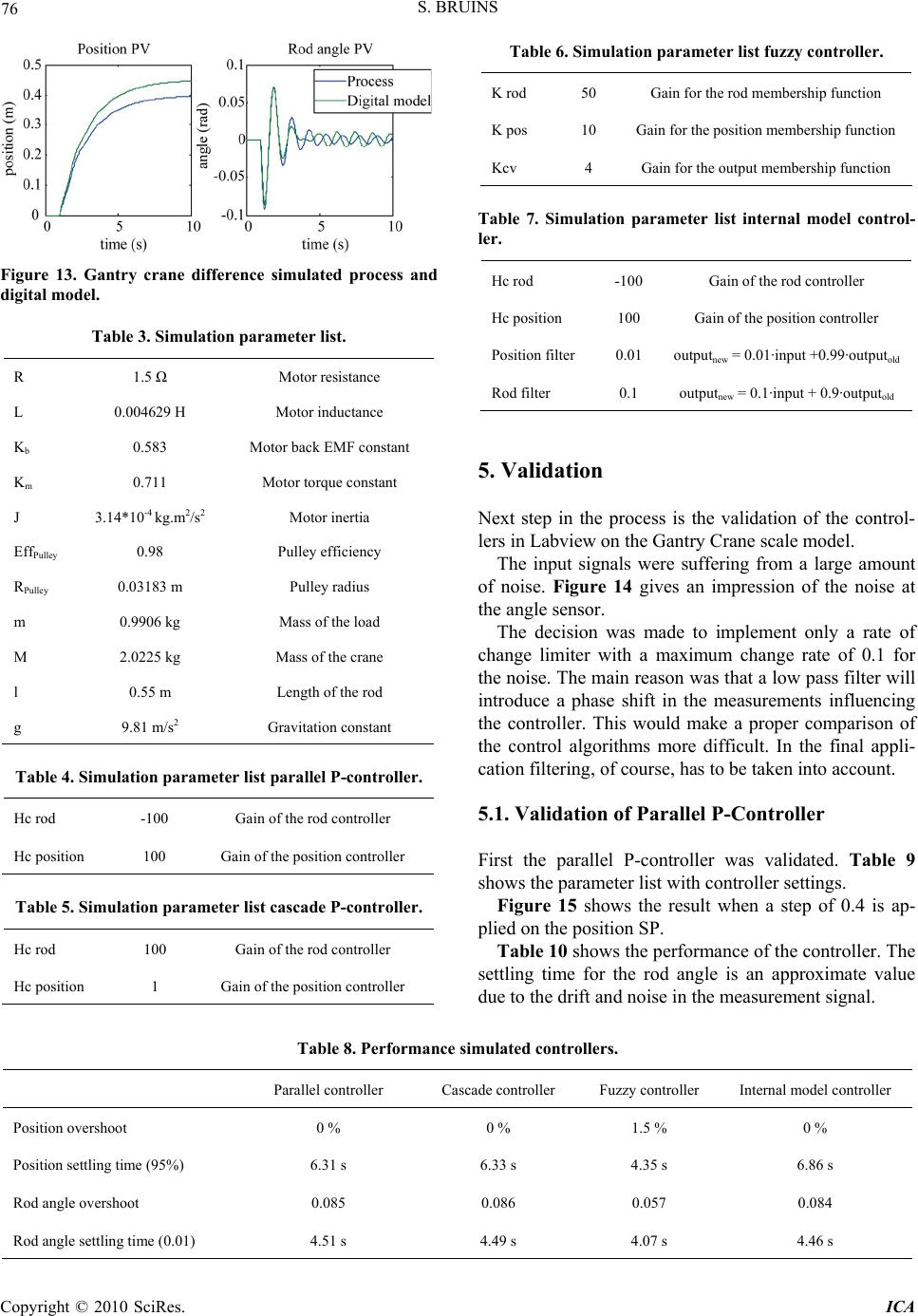

S. BRUINS
76
Figure 13. Gantry crane difference simulated process and
digital model.
Table 3. Simulation parameter list.
R 1.5 Ω Motor resistance
L 0.004629 H Motor inductance
Kb 0.583 Motor back EMF constant
Km 0.711 Motor torque constant
J 3.14*10-4 kg.m2/s2 Motor inertia
EffPulley 0.98 Pulley efficiency
RPulley 0.03183 m Pulley radius
m 0.9906 kg Mass of the load
M 2.0225 kg Mass of the crane
l 0.55 m Length of the rod
g 9.81 m/s2 Gravitation constant
Table 4. Simulation parameter list parallel P-controller.
Hc rod -100 Gain of the rod controller
Hc position 100 Gain of the position controller
Table 5. Simulation parameter list cascade P-controller.
Hc rod 100 Gain of the rod controller
Hc position 1 Gain of the position controller
Table 6. Simulation parameter list fuzzy controller.
K rod 50 Gain for the rod membership function
K pos 10 Gain for the position membership function
Kcv 4 Gain for the output membership function
Table 7. Simulation parameter list internal model control-
ler.
Hc rod -100 Gain of the rod controller
Hc position 100 Gain of the position controller
Position filter 0.01 outputnew = 0.01·input +0.99·outputold
Rod filter 0.1 outputnew = 0.1·input + 0.9·outputold
5. Validation
Next step in the process is the validation of the control-
lers in Labview on the Gantry Crane scale model.
The input signals were suffering from a large amount
of noise. Figure 14 gives an impression of the noise at
the angle sensor.
The decision was made to implement only a rate of
change limiter with a maximum change rate of 0.1 for
the noise. The main reason was that a low pass filter will
introduce a phase shift in the measurements influencing
the controller. This would make a proper comparison of
the control algorithms more difficult. In the final appli-
cation filtering, of course, has to be taken into account.
5.1. Validation of Parallel P-Controller
First the parallel P-controller was validated. Table 9
shows the parameter list with controller settings.
Figure 15 shows the result when a step of 0.4 is ap-
plied on the position SP.
Table 10 shows the performance of the controller. The
settling time for the rod angle is an approximate value
due to the drift and noise in the measurement signal.
Table 8. Performance simulated controllers.
Parallel controller Cascade controller Fuzzy controller Internal model controller
Position overshoot 0 % 0 % 1.5 % 0 %
Position settling time (95%) 6.31 s 6.33 s 4.35 s 6.86 s
Rod angle overshoot 0.085 0.086 0.057 0.084
Rod angle settling time (0.01) 4.51 s 4.49 s 4.07 s 4.46 s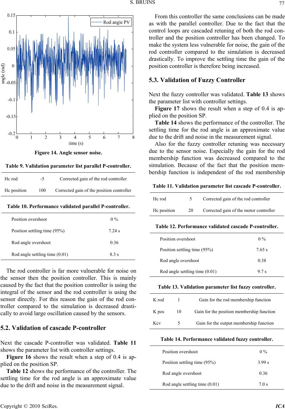

S. BRUINS
77
Figure 14. Angle sensor noise.
Table 9. Validation parameter list parallel P-controller.
Hc rod -5 Corrected gain of the rod controller
Hc position 100 Corrected gain of the position controller
Table 10. Performance validated parallel P-controller.
Position overshoot 0 %
Position settling time (95%) 7.24 s
Rod angle overshoot 0.36
Rod angle settling time (0.01) 8.3 s
The rod controller is far more vulnerable for noise on
the sensor then the position controller. This is mainly
caused by the fact that the position controller is using the
integral of the sensor and the rod controller is using the
sensor directly. For this reason the gain of the rod con-
troller compared to the simulation is decreased drasti-
cally to avoid large oscillation caused by the sensors.
5.2. Validation of cascade P-controller
Next the cascade P-controller was validated. Table 11
shows the parameter list with controller settings.
Figure 16 shows the result when a step of 0.4 is ap-
plied on the position SP.
Table 12 shows the performance of the controller. The
settling time for the rod angle is an approximate value
due to the drift and noise in the measurement signal.
From this controller the same conclusions can be made
as with the parallel controller. Due to the fact that the
control loops are cascaded retuning of both the rod con-
troller and the position controller has been changed. To
make the system less vulnerable for noise, the gain of the
rod controller compared to the simulation is decreased
drastically. To improve the settling time the gain of the
position controller is therefore being increased.
5.3. Validation of Fuzzy Controller
Next the fuzzy controller was validated. Table 13 shows
the parameter list with controller settings.
Figure 17 shows the result when a step of 0.4 is ap-
plied on the position SP.
Table 14 shows the performance of the controller. The
settling time for the rod angle is an approximate value
due to the drift and noise in the measurement signal.
Also for the fuzzy controller retuning was necessary
due to the sensor noise. Especially the gain for the rod
membership function was decreased compared to the
simulation. Because of the fact that the position mem-
bership function is independent of the rod membership
Table 11. Validation parameter list cascade P-controller.
Hc rod 5 Corrected gain of the rod controller
Hc position 20 Corrected gain of the motor controller
Table 12. Performance validated cascade P-controller.
Position overshoot 0 %
Position settling time (95%) 7.65 s
Rod angle overshoot 0.38
Rod angle settling time (0.01) 9.7 s
Table 13. Validation parameter list fuzzy controller.
K rod 1 Gain for the rod membership function
K pos 10 Gain for the position membership function
Kcv 5 Gain for the output membership function
Table 14. Performance validated fuzzy controller.
Position overshoot 0 %
Position settling time (95%) 3.99 s
Rod angle overshoot 0.36
Rod angle settling time (0.01) 7.0 s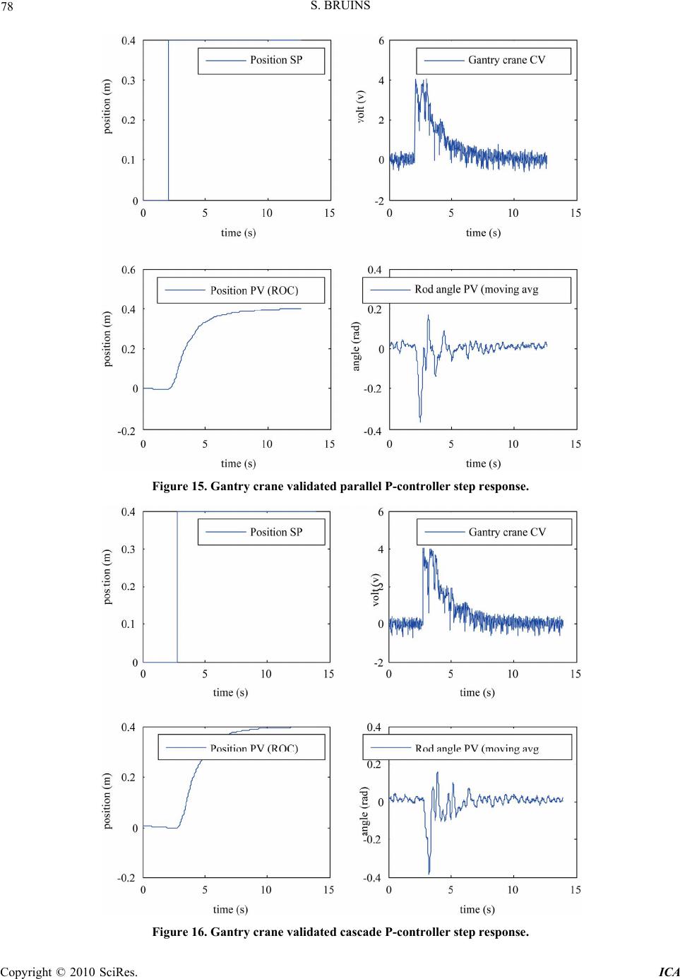

S. BRUINS
78
Figure 15. Gantry crane validated parallel P-controller step response.
Figure 16. Gantry crane validated cascade P-controller step response.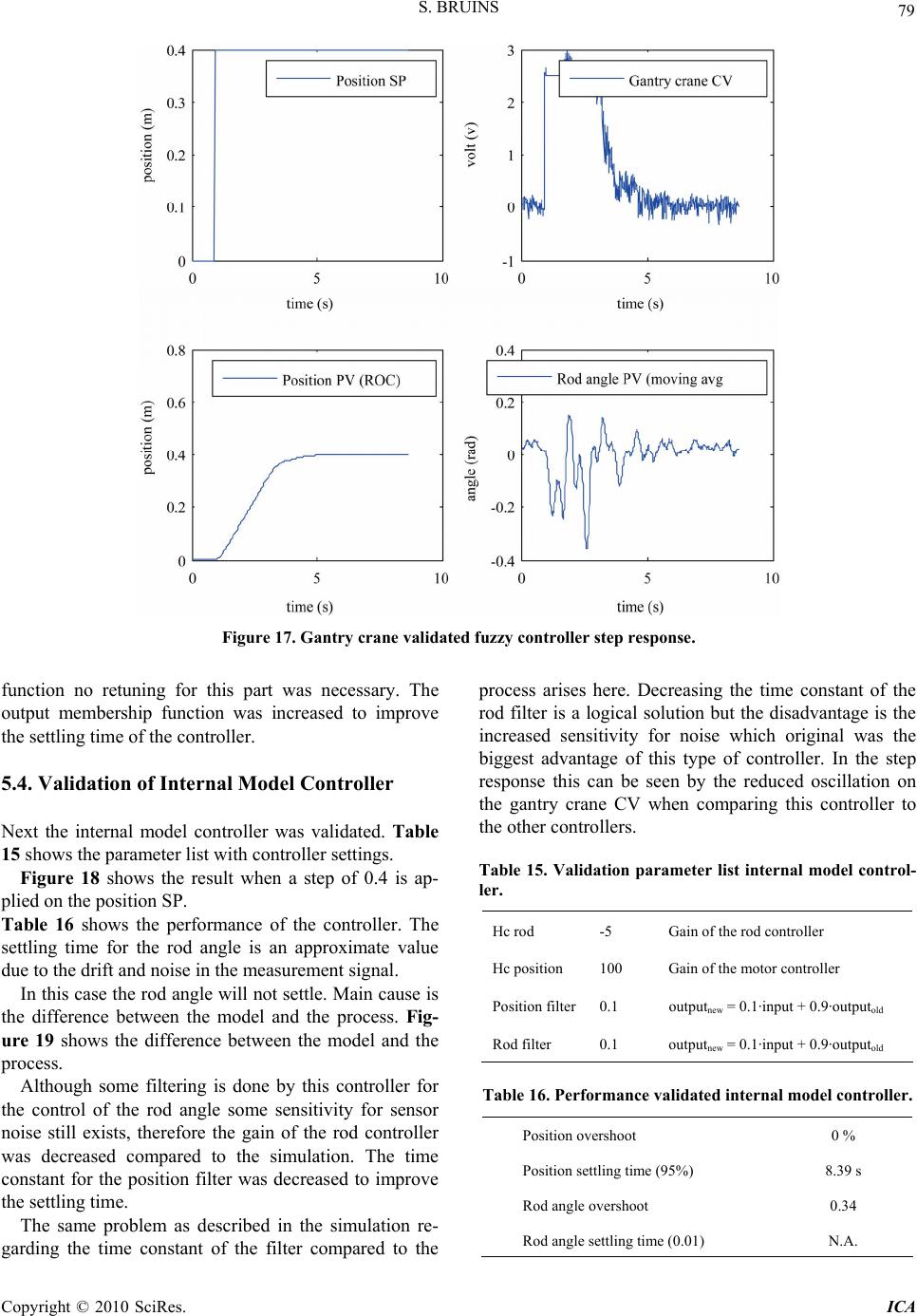

S. BRUINS
79
Figure 17. Gantry crane validated fuzzy controller step response.
function no retuning for this part was necessary. The
output membership function was increased to improve
the settling time of the controller.
5.4. Validation of Internal Model Controller
Next the internal model controller was validated. Table
15 shows the parameter list with controller settings.
Figure 18 shows the result when a step of 0.4 is ap-
plied on the position SP.
Table 16 shows the performance of the controller. The
settling time for the rod angle is an approximate value
due to the drift and noise in the measurement signal.
In this case the rod angle will not settle. Main cause is
the difference between the model and the process. Fig-
ure 19 shows the difference between the model and the
process.
Although some filtering is done by this controller for
the control of the rod angle some sensitivity for sensor
noise still exists, therefore the gain of the rod controller
was decreased compared to the simulation. The time
constant for the position filter was decreased to improve
the settling time.
The same problem as described in the simulation re-
garding the time constant of the filter compared to the
process arises here. Decreasing the time constant of the
rod filter is a logical solution but the disadvantage is the
increased sensitivity for noise which original was the
biggest advantage of this type of controller. In the step
response this can be seen by the reduced oscillation on
the gantry crane CV when comparing this controller to
the other controllers.
Table 15. Validation parameter list internal model control-
ler.
Hc rod -5 Gain of the rod controller
Hc position 100 Gain of the motor controller
Position filter0.1 outputnew = 0.1·input + 0.9·outputold
Rod filter 0.1 outputnew = 0.1·input + 0.9·outputold
Table 16. Performance validated internal model controller.
Position overshoot 0 %
Position settling time (95%) 8.39 s
Rod angle overshoot 0.34
Rod angle settling time (0.01) N.A.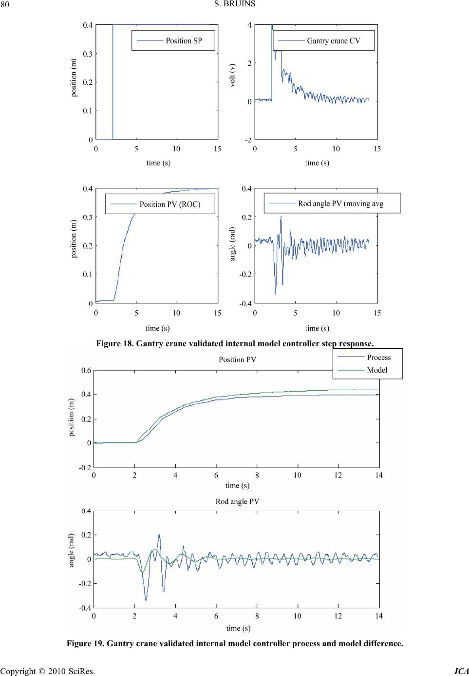

S. BRUINS
80
Figure 18. Gantry crane validated internal model controller step response.
Figure 19. Gantry crane validated internal model controller process and model difference.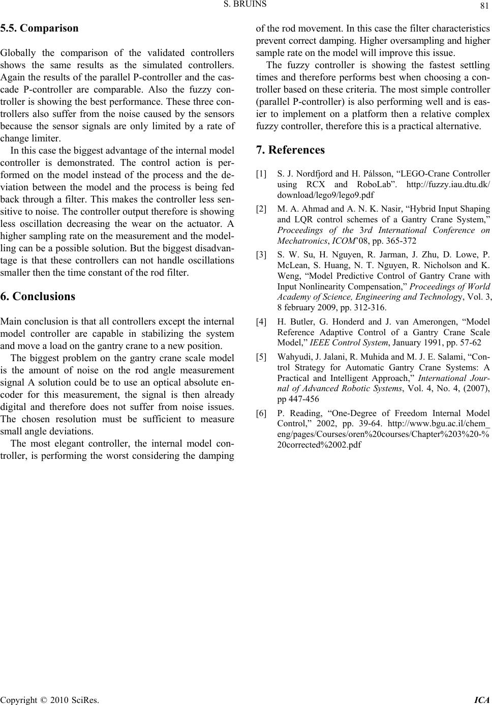

S. BRUINS
81
5.5. Comparison
Globally the comparison of the validated controllers
shows the same results as the simulated controllers.
Again the results of the parallel P-controller and the cas-
cade P-controller are comparable. Also the fuzzy con-
troller is showing the best performance. These three con-
trollers also suffer from the noise caused by the sensors
because the sensor signals are only limited by a rate of
change limiter.
In this case the biggest advantage of the internal model
controller is demonstrated. The control action is per-
formed on the model instead of the process and the de-
viation between the model and the process is being fed
back through a filter. This makes the controller less sen-
sitive to noise. The controller output therefore is showing
less oscillation decreasing the wear on the actuator. A
higher sampling rate on the measurement and the model-
ling can be a possible solution. But the biggest disadvan-
tage is that these controllers can not handle oscillations
smaller then the time constant of the rod filter.
6. Conclusions
Main conclusion is that all controllers except the internal
model controller are capable in stabilizing the system
and move a load on the gantry crane to a new position.
The biggest problem on the gantry crane scale model
is the amount of noise on the rod angle measurement
signal A solution could be to use an optical absolute en-
coder for this measurement, the signal is then already
digital and therefore does not suffer from noise issues.
The chosen resolution must be sufficient to measure
small angle deviations.
The most elegant controller, the internal model con-
troller, is performing the worst considering the damping
of the rod movement. In this case the filter characteristics
prevent correct damping. Higher oversampling and higher
sample rate on the model will improve this issue.
The fuzzy controller is showing the fastest settling
times and therefore performs best when choosing a con-
troller based on these criteria. The most simple controller
(parallel P-controller) is also performing well and is eas-
ier to implement on a platform then a relative complex
fuzzy controller, therefore this is a practical alternative.
7. References
[1] S. J. Nordfjord and H. Pálsson, “LEGO-Crane Controller
using RCX and RoboLab”. http://fuzzy.iau.dtu.dk/
download/lego9/lego9.pdf
[2] M. A. Ahmad and A. N. K. Nasir, “Hybrid Input Shaping
and LQR control schemes of a Gantry Crane System,”
Proceedings of the 3rd International Conference on
Mechatronics, ICOM’08, pp. 365-372
[3] S. W. Su, H. Nguyen, R. Jarman, J. Zhu, D. Lowe, P.
McLean, S. Huang, N. T. Nguyen, R. Nicholson and K.
Weng, “Model Predictive Control of Gantry Crane with
Input Nonlinearity Compensation,” Proceedings of World
Academy of Science, Engineering and Technology, Vol. 3,
8 february 2009, pp. 312-316.
[4] H. Butler, G. Honderd and J. van Amerongen, “Model
Reference Adaptive Control of a Gantry Crane Scale
Model,” IEEE Control System, January 1991, pp. 57-62
[5] Wahyudi, J. Jalani, R. Muhida and M. J. E. Salami, “Con-
trol Strategy for Automatic Gantry Crane Systems: A
Practical and Intelligent Approach,” International Jour-
nal of Advanced Robotic Systems, Vol. 4, No. 4, (2007),
pp 447-456
[6] P. Reading, “One-Degree of Freedom Internal Model
Control,” 2002, pp. 39-64. http://www.bgu.ac.il/chem_
eng/pages/Courses/oren%20courses/Chapter%203%20-%
20corrected%2002.pdf