Creative Education
2013. Vol.4, No.5, 340-347
Published Online May 2013 in SciRes (http://www.scirp.org/journal/ce) http://dx.doi.org/10.4236/ce.2013.45050
Copyright © 2013 SciRes.
340
The Analysis and Reporting of the Dundee Ready
Education Environment Measure (DREEM):
Some Informed Guidelines for Evaluators
Louise Swift, Susan Miles, Sam J. Leinster
Norwich Medical School, Faculty of Medicine and Health Sciences, University of East Anglia, Norwich, UK
Email: L.Swift@uea.ac.uk
Received March 23rd, 2013; revised April 25th, 2013; accepted May 8th, 2013
Copyright © 2013 Louise Swift et al. This is an open access article distributed under the Creative Commons At-
tribution License, which permits unrestricted use, distribution, and reproduction in any medium, provided the
original work is properly cited.
Background: There is a need to evaluate perceptions of the educational environment of training institu-
tions for health professionals as part of any assessment of quality standards for education. The Dundee
Ready Education Environment Measure (DREEM) is a widely used tool for evaluating the educational
environment of medical and other health schools. However, methods of analysis reported in the published
DREEM literature are inconsistent which could lead to misinterpretation of areas for change and, addi-
tionally, this makes comparison between institutions difficult. Those involved in course evaluation are
usually not statisticians and there are no guidelines on DREEM’s reporting or statistical analysis. This
paper aims to clarify the choice of methods for the analysis of the DREEM. Method: The statistical lit-
erature, typical properties of DREEM data and the results from a series of statistical simulations were
used to inform our recommendations. Results: We provide a set of guidelines for the analysis and report-
ing of the DREEM. In particular, we provide evidence that when comparing independent samples of
Likert response data similar to that generated by the DREEM, the non-parametric Wilcoxon Mann Whit-
ney test performs well. Further, one should be wary of using non-parametric methods on matched samples
of such data as they may be overly ready to reject null hypothesis. Conclusions: Our recommendations
have the potential to improve the accuracy and consistency with which the inadequacies in the medical
school environment can be identified and assess the success of any changes. They should also facilitate
comparison between different institutions using the DREEM.
Keywords: DREEM; Likert; Educational Environment; Evaluation; Medical Education; Simulation;
Statistical Test
Introduction
The educational environment of a medical school is both a
“manifestation of the curriculum” and a “determinant… of the
behaviour of the medical school’s students and teachers” (Genn,
2001a: p 342). Genn (2001b) argues that perceptions of the
educational environment (the “climate”) influence student satis-
faction, and student achievement and success. Given its impor-
tance and the fact that the educational environment can be
changed, it is imperative to measure it; and in so doing, to di-
agnose strengths and weaknesses that can be remediated to
ensure a high quality learning experience for students.
The Dundee Ready Education Environment Measure
(DREEM) was designed to measure the educational environ-
ment specifically for medical schools and schools for other
health professions (Roff et al., 1997). A recent review of the
literature to identify and assess instruments designed to meas-
ure the educational environment of different health professional
training settings concluded that the DREEM was the most suit-
able instrument for the undergraduate medical education setting
(Soemantri et al., 2010). The DREEM is comprised of 50 items,
each with a five-point Likert response (“Strongly Agree” (4),
“Agree” (3), “Unsure” (2), “Disagree” (1) and “Strongly Dis-
agree” (0)). The items can be examined individually, combined
into five subscales or a total DREEM score. Although the au-
thors of the DREEM give guidelines for its interpretation, they
do not advise on appropriate methods of statistical inference
(McAleer & Roff, 2001). An extensive review of the published
literature since the DREEM was introduced in Roff et al.’s
1997 publication showed that the DREEM has been widely
utilised in a variety of settings at a worldwide level, indicating
that it is a valued and useful tool by many health professional
training institutions; however, the methods of analysis and re-
porting are far from consistent (Miles et al., 2012).
Our aim was to provide a set of recommendations for the
analysis and reporting of the DREEM. This would enable the
DREEM to be used more easily by evaluators, to more accu-
rately identify problem areas and to facilitate comparison be-
tween institutions. However, there is controversy about how
Likert data should be analysed that must be taken into account
when considering how best to analyse DREEM data.
First, there is debate about the validity of taking a Likert re-
sponse and treating it as numerical (see, for example, Carifio,
2007). However, the authors of the DREEM intended the item
L. SWIFT ET AL.
scores to be used and combined as numbers so this question can
be put aside for the DREEM. Second, there is controversy as to
whether it is reasonable to treat Likert response scores as con-
tinuous numerical data, also known as interval data, which
opens up the possibility of using parametric methods. Jamieson
(2004) provoked considerable discussion by arguing that as
Likert scales are ordinal they should never be analysed using
parametric methods, because parametric methods make as-
sumptions such as the normality of the data. However, Carifio
(2007, 2008) makes the important distinction between a single
Likert item and a Likert scale, that is a collection of Likert
items, and supports the case that it is reasonable to treat a com-
bination of eight or more items as interval data; which would
apply in the case of the whole 50 item DREEM or its mul-
ti-item subscales. Third, Carifio (2008) also argues that single
items of a measurement scale should rarely be analysed alone
because they form part of a “structured and reasoned whole”.
However, the authors of DREEM call it a “diagnostic tool” and
the developers intended each item of the DREEM to be used
individually to diagnose problems in that area. As such, we
argue that it is valid to consider each item individually, as well
as looking at the five subscales and the full DREEM instrument.
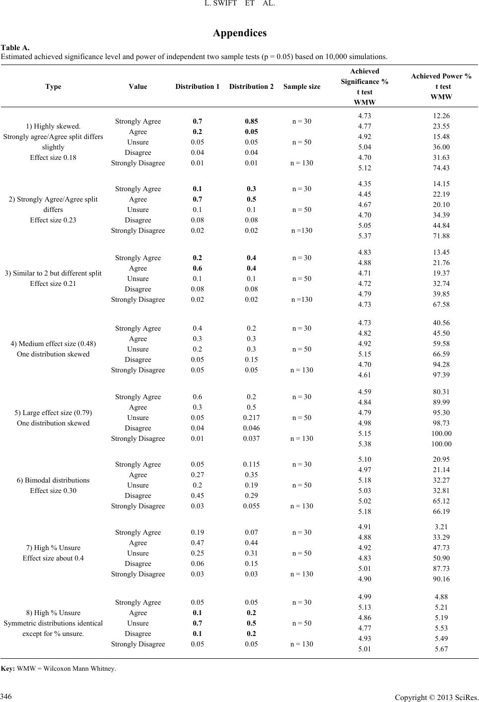
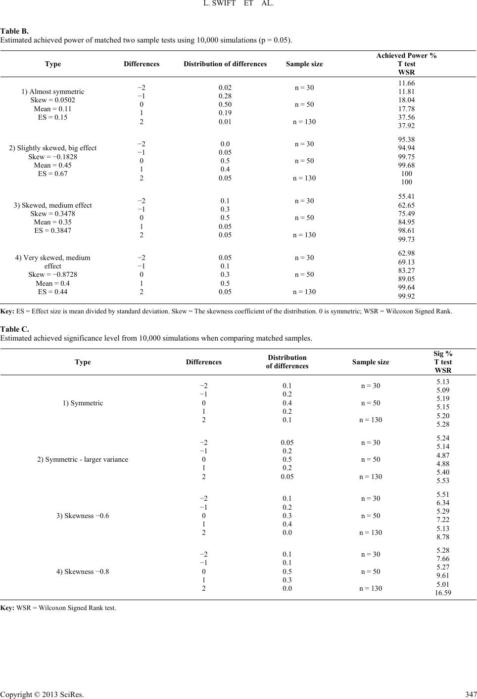
This led us to our own investigations, using a series of simu-
lations to assess the performance of candidate statistical tests
for the Likert data generated by the DREEM. Our aim was that
these simulations would inform a set of recommendations for
the analysis and reporting of the DREEM for current and future
users of the DREEM. The investigations also have wider re-
percussions, in that they are applicable to Likert responses in
general.
Methodology
Information from the articles reviewed by Miles et al. (2012)
and unpublished student evaluation data from the Norwich
Medical School, University of East Anglia (UEA) was used to
identify typical distributions for the item responses. We then
ran a series of simulations in Stata v8 to assess the performance,
for data of this kind, of alternative tests suggested by the statis-
tical literature. A sample size of 30 was used to reflect the con-
ventional threshold at which a parametric test is applied to
non-normal samples and 50 and 130 to represent a subgroup of
a year group and a whole year group of students respectively.
The Distribution of Individual DREEM Responses
Data from UEA and research publications suggest that a
common distribution of responses for a single DREEM item is
50% - 70% Agreeing, 40% - 20% Strongly Agreeing with the
remaining small percentage spread between Strongly Disagree,
Disagree and Unsure resulting in a skewed distribution. Further,
as Till (2004) points out, a great number of items have bimodal
distributions, that is, a high percentage disagree and a high
percentage agree giving “mixed messages”. Another common
occurrence is to observe a very high percentage of Unsure an-
swers, with smaller percentages agreeing or disagreeing. Any
method of reporting and analysis must therefore be suitable for
all these types of distribution.
The Uses of the DREEM
Miles et al. (2012) identified three main uses of the DREEM
for evaluation purposes. First, it is used as a diagnostic tool;
that is to highlight elements of a course/curriculum which are
currently unsatisfactory and need remediation. Second, it can be
used to compare two or more completely separate groups of
students, for instance, males with females or one year group
with another. More generally this is known as the independent
samples case. Third, it is used to compare the same group of
students on different occasions; the matched case. This might
be, for instance, to compare a cohort’s experiences from one
academic year to another or alternatively to compare a group of
students’ scores with their “ideal” or “expected” score. We will
consider each of these in turn.
The DREEM as a Diagnostic Tool
Considerations
The developers suggest reporting mean scores across all par-
ticipants for each of the 50 items separately. If using the
DREEM for purely diagnostic purposes examination of these
means will indicate areas of strength and weakness. Individual
items with a mean score of 3.5 are particularly strong areas,
items with a mean score of 2.0 need particular attention, and
items with mean scores between 2 and 3 are areas of the educa-
tional environment that could be improved (McAleer and Roff,
2001).
Recommendations
It is certainly meaningful to use means rather than medians
because the median can only take one of the five possible
scores. However, for skewed or bimodal distributions, which
commonly occur in the DREEM, an item with an acceptable
central measure may still mask a high proportion of negative
responses, so this alone does not seem adequate. We therefore
suggest reporting a table of results which summarises the re-
sponses by merging the Agree/Strongly Agree, Disagree/
Strongly Disagree categories and reports the mean. Further we
propose using a series of warnings or “flags”, with thresholds
decided a priori to alert to items with a low percentage agree-
ment, a high percentage unsure and/or a high percentage dis-
agree as well as means below a particular level, say 2.0 as rec-
ommended by the developers or 2.5 if one wants to be stricter.
Given that many items give skewed responses the standard
deviation can mislead, so we do not recommend its inclusion.
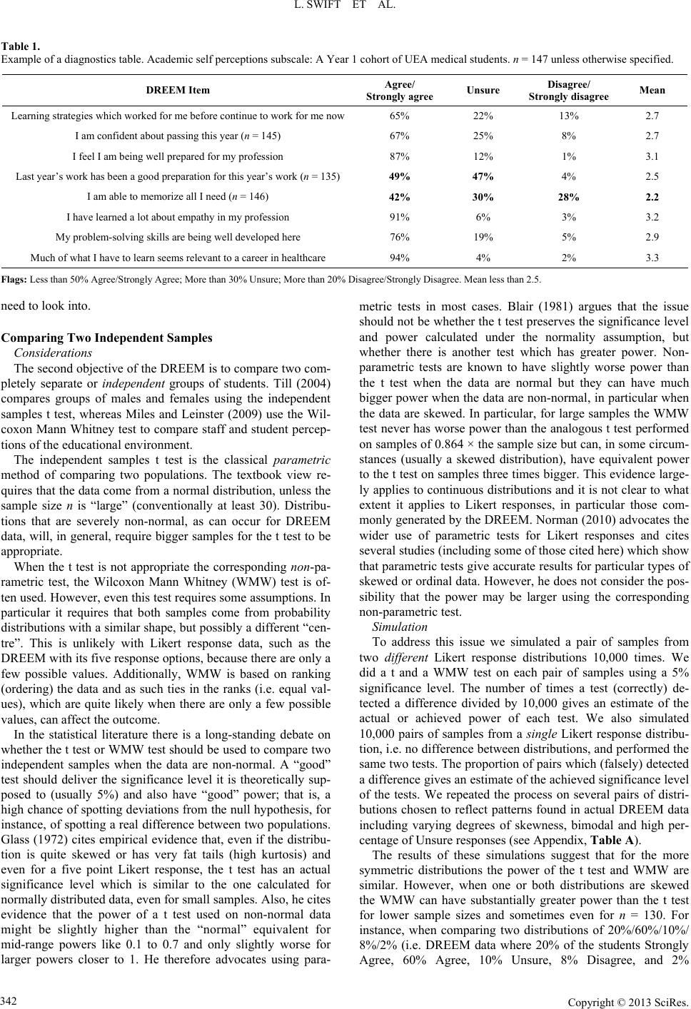
An example for one of the DREEM’s five subscales using
data from Year 1 UEA medical students can be seen in Table 1.
We have flagged in bold those items where less than 50% of
students Agree/Strongly Agree, more than 30% are Unsure and
more than 20% Disagree/Strongly Disagree. Notice that flags
occur on the items “Last year’s work has been a good prepara-
tion for this year’s work” and “I am able to memorize all I
need”. Whilst the item “Last year’s work has been a good
preparation for this year’s work” has a low but acceptable mean
of 2.5 the “flag” system draws attention to the fact that less than
50% of respondents agree and nearly all the others are unsure
suggesting that this is an item that needs attention from the
teaching team. However, in this case we would not necessarily
expect first year students to feel that the work they had done
last year (for instance A levels, an Access to Medicine course
or employment) was a good preparation for their first year of
medical school and there is no cause for concern. This illus-
trates the importance of interpreting the DREEM scores ac-
cording to their unique situational context at each educational
institution. In contrast, the flag for the item “I am able to mem-
orize all I need” suggests that there may be a concern about
workload or learning strategies that the teaching team might
Copyright © 2013 SciRes. 341
L. SWIFT ET AL.
Copyright © 2013 SciRes.
342
Table 1.
Example of a diagnostics table. Academic self perceptions subscale: A Year 1 cohort of UEA medical students. n = 147 unless otherwise specified.
DREEM Item Agree/
Strongly agree Unsure Disagree/
Strongly disagree Mean
Learning strategies which worked for me before continue to work for me now65% 22% 13% 2.7
I am confident about passing this year (n = 145) 67% 25% 8% 2.7
I feel I am being well prepared for my profession 87% 12% 1% 3.1
Last year’s work has been a good preparation for this year’s work (n = 135) 49% 47% 4% 2.5
I am able to memorize all I need (n = 146) 42% 30% 28% 2.2
I have learned a lot about empathy in my profession 91% 6% 3% 3.2
My problem-solving skills are being well developed here 76% 19% 5% 2.9
Much of what I have to learn seems relevant to a career in healthcare 94% 4% 2% 3.3
Flags: Less than 50% Agree/Strongly Agree; More than 30% Unsure; More than 20% Disagree/Strongly Disagree. Mean less than 2.5.
need to look into.
Comparing Two Independent Sample s
Considerations
The second objective of the DREEM is to compare two com-
pletely separate or independent groups of students. Till (2004)
compares groups of males and females using the independent
samples t test, whereas Miles and Leinster (2009) use the Wil-
coxon Mann Whitney test to compare staff and student percep-
tions of the educational environment.
The independent samples t test is the classical parametric
method of comparing two populations. The textbook view re-
quires that the data come from a normal distribution, unless the
sample size n is “large” (conventionally at least 30). Distribu-
tions that are severely non-normal, as can occur for DREEM
data, will, in general, require bigger samples for the t test to be
appropriate.
When the t test is not appropriate the corresponding non-pa-
rametric test, the Wilcoxon Mann Whitney (WMW) test is of-
ten used. However, even this test requires some assumptions. In
particular it requires that both samples come from probability
distributions with a similar shape, but possibly a different “cen-
tre”. This is unlikely with Likert response data, such as the
DREEM with its five response options, because there are only a
few possible values. Additionally, WMW is based on ranking
(ordering) the data and as such ties in the ranks (i.e. equal val-
ues), which are quite likely when there are only a few possible
values, can affect the outcome.
In the statistical literature there is a long-standing debate on
whether the t test or WMW test should be used to compare two
independent samples when the data are non-normal. A “good”
test should deliver the significance level it is theoretically sup-
posed to (usually 5%) and also have “good” power; that is, a
high chance of spotting deviations from the null hypothesis, for
instance, of spotting a real difference between two populations.
Glass (1972) cites empirical evidence that, even if the distribu-
tion is quite skewed or has very fat tails (high kurtosis) and
even for a five point Likert response, the t test has an actual
significance level which is similar to the one calculated for
normally distributed data, even for small samples. Also, he cites
evidence that the power of a t test used on non-normal data
might be slightly higher than the “normal” equivalent for
mid-range powers like 0.1 to 0.7 and only slightly worse for
larger powers closer to 1. He therefore advocates using para-
metric tests in most cases. Blair (1981) argues that the issue
should not be whether the t test preserves the significance level
and power calculated under the normality assumption, but
whether there is another test which has greater power. Non-
parametric tests are known to have slightly worse power than
the t test when the data are normal but they can have much
bigger power when the data are non-normal, in particular when
the data are skewed. In particular, for large samples the WMW
test never has worse power than the analogous t test performed
on samples of 0.864 × the sample size but can, in some circum-
stances (usually a skewed distribution), have equivalent power
to the t test on samples three times bigger. This evidence large-
ly applies to continuous distributions and it is not clear to what
extent it applies to Likert responses, in particular those com-
monly generated by the DREEM. Norman (2010) advocates the
wider use of parametric tests for Likert responses and cites
several studies (including some of those cited here) which show
that parametric tests give accurate results for particular types of
skewed or ordinal data. However, he does not consider the pos-
sibility that the power may be larger using the corresponding
non-parametric test.
Simulation
To address this issue we simulated a pair of samples from
two different Likert response distributions 10,000 times. We
did a t and a WMW test on each pair of samples using a 5%
significance level. The number of times a test (correctly) de-
tected a difference divided by 10,000 gives an estimate of the
actual or achieved power of each test. We also simulated
10,000 pairs of samples from a single Likert response distribu-
tion, i.e. no difference between distributions, and performed the
same two tests. The proportion of pairs which (falsely) detected
a difference gives an estimate of the achieved significance level
of the tests. We repeated the process on several pairs of distri-
butions chosen to reflect patterns found in actual DREEM data
including varying degrees of skewness, bimodal and high per-
centage of Unsure responses (see Appendix, Table A).
The results of these simulations suggest that for the more
symmetric distributions the power of the t test and WMW are
similar. However, when one or both distributions are skewed
the WMW can have substantially greater power than the t test
for lower sample sizes and sometimes even for n = 130. For
instance, when comparing two distributions of 20%/60%/10%/
8%/2% (i.e. DREEM data where 20% of the students Strongly
Agree, 60% Agree, 10% Unsure, 8% Disagree, and 2%
L. SWIFT ET AL.
Strongly Disagree) and 40%/40%/10%/8%/2% respectively for
a sample size of 130 in each group the t test had an estimated
achieved power of 40% and the WMW 68% (simulation 3 of
Table A).
We should emphasise (illustrated in the final simulation of
Table A) that these tests cannot detect different distributions if
the mean/medians are similar. We therefore suggest comparing
the percentages of respondents who disagree (i.e. Disagree/
Strongly Disagree) using a chi squared test. Note that chi
squared tests comparing three or more categories between
groups are not appropriate as the data are ordinal, not nominal.
Power calculations using standard sample size software suggest
that it is feasible to use a chi squared analysis on a whole year
group of students (n = 130) but not on sub-groups within a year
group. For instance (using nquery), if in one year 50% of re-
spondents Disagreed/Strongly Disagreed a chi squared test to
detect a 20 percentage point difference the following year
would have a power of 91% for n = 130 but only 53% for n = 50.
Multiple tests
If every DREEM item is analysed individually 50 separate
significance tests will be performed. If the significance level is
5%, it can be shown mathematically that there is a 92% chance
that at least one is significant, when no real difference exist. A
classical solution to this, known as Bonferroni’s correction, is
to divide the significance level by the number of tests. However,
this is known to be conservative and it increases the probability
of missing a real difference. Another school of thought advo-
cates reducing the number of outcomes under study and inter-
preting the results of statistical tests in the context of the quality
of the study and the size of the finding (e.g. Feise, 2002). For
the DREEM this might mean including in the main analysis only
those items identified previously as requiring remedial action.
Recommendations
Table 2 demonstrates our recommendations, informed by the
simulations, for comparing two independent samples of
DREEM responses. It uses data from UEA Year 1 and Year 2
medical students on the DREEM’s Academic self perceptions
subscale. We suggest reporting the results of the DREEM in a
table summarising the responses using the percentage Strongly
Agree/Agree; Unsure, and Strongly Disagree/Disagree for each
group, the two means, the mean difference and then the results
of both a t test and a Wilcoxon Mann Whitney test. We would
also include a chi squared test of the difference in the percent-
age who Strongly Disagree/Disagree (it would be equally valid
to do a chi squared test of the difference in the percentage who
Strongly Agree/Agree). A rule of thumb for the validity of the
chi squared test is that np and n(1 – p), where p is the observed
proportion over both groups, are both 5 or more. We therefore
suggest exercising caution and not performing the test where an
observed percentage is, say, less than 5%. Significance on any
test would be flagged, without any adjustment for multiple
comparisons. And, as in the diagnostic Table 1, low percentage
agreement, high unsure, high disagreement and low means
would also be flagged.
Notice that both the t and WMW tests are significant for the
items “Much of what I have to learn seems relevant to a career
in healthcare”, “I am able to memorize all I need”, “I am con-
fident about passing this year” and “Learning strategies which
worked for me before continue to work for me now”; but for
the item, “Last year’s work has been a good preparation for this
year” the WMW is highly significant whereas the t test is not
significant. On inspection this latter item is highly skewed
which explains why WMW has detected a difference but the t
test has not, as suggested by the simulations.
Comparing Two Matched Samples
Considerations
Matched samples arise when two sets of responses are ob-
tained for the same group of individuals, for instance at two
separate points in time; the scores of interest are the set of
change scores. For DREEM, matched data also arise when
student expectations of the environment are compared with
Table 2.
Example of a table for comparing two independent samples. Academic self perceptions subscale comparing two different cohorts of UEA medical
students.
Year 1 Year 2 Year 1 Year 2
DREEM Item nSA/A Unsure SD/Dn SA/AUnsureSD/DChi sq (SD/D)Mean Mean T testWMW
Learning strategies which worked
for me before continue to work for
me now
14765% 22% 13% 14257%23% 19% 0.157 2.7 2.4 0.0140.020
I am confident about passing this
year 14567% 25% 8%14255%34% 11% 0.372 2.7 2.5
0.0340.016
I feel I am being well prepared for
my profession 14787% 12% 1%14282%13% 5% - 3.1 3.0 0.1140.167
Last year’s work has been a good
preparation for this year’s work 135 49% 47% 4%14271%18% 11% - 2.5 2.7 0.0650.006
I am able to memorize all I need 14642% 30% 28% 142 35% 25% 39% 0.038 2.2 1.9 0.0270.040
I have learned a lot about empathy
in my profession 14791% 6% 3% 14291%3% 6% - 3.2 3.1 0.1430.191
My problem-solving skills are
being well developed here 14776% 19% 5%14284%12% 4% - 2.9 3.0 0.5840.694
Much of what I have to learn seems
relevant to a career in healthcare 14794% 4% 2%142 89%6% 5% - 3.3 3.1 0.0080.008
SA/A = Strongly Agree/Agree; SD/D = Strongly Disagree/Disagree; Chi square test between percentage Strongly disagree/Disagree where both percentages are >5% only;
Flags: Less than 50% Agree/Strongly Agree; More than 30% Unsure; More than 20% Disagree/Strongly Disagree. Mean less than 2.5.
Copyright © 2013 SciRes. 343
L. SWIFT ET AL.
their actual perceptions at the end of that year (e.g. Miles &
Leinster, 2007). The amount by which the actual scores fall-
short of the expected is termed the “dissonance”. Till (2005)
reports items with the largest dissonance and uses the paired
sample t test. Miles and Leinster (2007) report the average dis-
sonance for each item of the DREEM and then use a Wilcoxon
Signed Rank (WSR) test to test whether the subscales have zero
median dissonance.
The paired samples t test is equivalent to a single sample t
test in that the changes have zero mean. It assumes that the
changes are normally distributed but, as for the independent
samples t test, this condition can be waived for “large” samples.
The WSR is a non-parametric test, but still assumes that the
distribution of the changes is symmetric. Glass (1972: p. 262)
gives a table from Srivastava (1959) reporting the theoretical
power of the t test if it is conducted on small samples of data (n
= 10) with various types of non-normality. The power, unless it
is low, is very similar to that of normal data; supporting the use
of the t test.
Simulation
To investigate the power of the two types of test we simu-
lated 10,000 samples from each of four possible change distri-
butions. These distributions were chosen to be typical of the
distributions of the changes and dissonances found in actual
DREEM data and to have non-zero means and varying degrees
of symmetry/skewness (see Appendix, Table B). Again the
proportion of simulated samples which detect a non-zero mean
change gives an estimate of the power of each of the tests. The
results suggest that the two types of test have similar power for
more symmetric distributions but the WSR has slightly better
power for skewed distributions unless the power approaches
100%. For instance, if 10% of the changes are 2, 30% are 1,
50% are 0 and 5% are 1 and 2, i.e. a skewed distribution with
effect size about 0.4, the power of the t test is 75% and of the
WSR is 85% for a sample size of 50 (simulation 3 of Appendix,
Table B).
The achieved significance level of these tests depends on the
exact distribution of the changes under the null hypothesis of a
zero mean/median. To estimate this we simulated 10,000 sam-
ples from several zero mean distributions with varying skew-
ness (see Appendix, Table C). The results indicated that for the
symmetric distributions both tests give achieved significance
levels which are approximately 5% as desired. However, for
skewed distributions the WSR test appears more likely to in-
correctly detect a change than it should be. For instance, for a
moderately skewed distribution (40% of the changes are 1, 30%
zero, 20% 1 and 10% 2) 8.8% of samples of size 130 give a
significant results when the WSR is used, but only 5.3% with
the t test (simulation 3 of Appendix, Table C).
Note that the chi squared test is not a valid test to compare
percentages of matched data as the same students are contrib-
uting scores into both data sets. McNemar’s test of equal pro-
portions is appropriate (e.g. Agresti 2002, page 411).
Recommendations
These findings lead us to suggest producing a similar table to
Table 2 (for comparing two independent samples) for matched
data but reporting only the t test and using McNemar instead of
the chi squared test (example table not provided due to the
similarity to Table 2).
Subscales and Total Scores
Subscale scores of the DREEM are constructed by adding up
responses from the seven to twelve individual items making up
the subscale. As with the individual items, the developers give
guidance on interpreting the score for each subscale and total
(McAleer & Roff, 2001) but none on statistical inference. Sta-
tistically, whilst sums of independent items are likely to be
“more” normally distributed than the items themselves, items
which have been grouped into subscales are likely to be mutu-
ally correlated and so there may still be strong non-normality.
We therefore advocate treating the subscale results in much the
same way as the individual items; that is performing both t and
non-parametric tests on independent samples case but only t
tests on matched samples. However, as subscale scores can take
a large number of possible values the median could be reported
as well as the mean. For consistency of presentation we would
recommend reporting total DREEM scores in a similar way.
Discussion and Conclusion
Methods for the analysis and reporting of the DREEM have
not been consistent in the medical education research literature
and more generally there has been controversy on how Likert
response data should be analysed. The results of our simula-
tions have led to these guidelines for the analysis and reporting
of DREEM data. However, the results of our simulations are
applicable to Likert responses in general and support the view
that when comparing independent samples, in particular those
from skewed or bimodal distributions, the non-parametric
WMW test performs well and may have greater power than the
t test. However, one should be wary of using non-parametric
methods on matched samples as they may be overly ready to
reject null hypotheses.
We have not explicitly considered the comparison of three or
more independent samples (for example DREEM data from all
years of five year medical course). The selection of three or
more distributions for simulation under the alternative hypothe-
sis is impractical as there is a plethora of possibilities; so we
have not run simulations for such comparisons. However, our
view would be to use the analogue of the independent samples t
test and WMW tests; that is analysis of variance and the non-
parametric equivalent, Kruskall Wallis, in a similar way to the
two sample situation.
The recommendations we have given will make it easier for
those involved in evaluation to report and analyse the DREEM.
This should allow medical schools to use the DREEM to more
accurately identify areas for change and assess the success of
consequent changes. Further, greater standardisation of method
should facilitate comparison between medical schools. More
generally, the simulation results add to the understanding of
how to analyse individual Likert responses, a subject of some
contention.
REFERENCES
Agresti, A. (2002). Categorical data analysis. 2nd Edition, Hoboken,
NJ: Wiley. doi:10.1002/0471249688
Blair, R. C. (1981). A reaction to “Consequences of failure to meet
assumptions underlying the fixed effects analysis of variance and
covariance”. Review of Educational Research, 51, 499-507.
doi:10.3102/00346543051004499
Carifio, J., & Perla, R. J. (2007). Ten common misunderstandings, mis-
conceptions, persistent myths and urban legends about Likert scales
and Likert response formats and their antidotes. Journal of Social
Sciences, 3, 106-116.
Copyright © 2013 SciRes.
344
L. SWIFT ET AL.
Carifio, J., & Perla, R. J. (2008). Resolving the 50-year debate around
using and misusing Likert scales. Medical Education, 42, 1150-1152.
doi:10.1111/j.1365-2923.2008.03172.x
Feise, R. J. (2002). Do multiple outcome measures require p-value ad-
justment? BMC Medical Research Methodology, 2, 8.
doi:10.1186/1471-2288-2-8
Genn, J. M. (2001a). AMEE Medical Education Guide No. 23 (Part 1).
Curriculum, environment, climate, quality and change in medical
education: A unifying perspective. Medical Teacher, 23, 337-344.
doi:10.1080/01421590120063330
Genn, J. M. (2001b). AMEE Medical Education Guide No. 23 (Part 2).
Curriculum, environment, climate, quality and change in medical
education: A unifying perspective. Medical Teacher, 23, 445-454.
Glass, G. V., Peckham, P. D., & Sanders, J. R. (1972). Consequences of
failure to meet assumptions underlying the fixed effects analysis of
variance and covariance. Review of Educational Research, 42, 237-
288. doi:10.3102/00346543042003237
Jamieson, S. (2004). Likert scales: How to (ab)use them. Medical Edu-
cation, 38, 1212-1218. doi:10.1111/j.1365-2929.2004.02012.x
McAleer, S., & Roff, S. (2001). A practical guide to using the Dundee
Ready Education Environment Measure (DREEM). In J. M. Genn
(Ed.), Curriculum, environment, climate, quality and change in me-
dical education: A unifying perspective (pp. 29-33). AMEE Educa-
tion Guide no. 23. Scotland: AMEE.
Miles, S., & Leinster, S. J. (2007). Medical students’ perceptions of
their educational environment: Expected versus actual perceptions.
Medical Education, 4 1, 265-272.
doi:10.1111/j.1365-2929.2007.02686.x
Miles, S., & Leinster, S. J. (2009). Comparing staff and student percep-
tions of the student experience at a new medical school. Medical
Teacher, 31, 539-546. doi:10.1080/01421590802139732
Miles, S., Swift, L., & Leinster, S. J. (2012). The Dundee Ready Edu-
cation Environment Measure (DREEM): A review of its adoption
and use. Medical Teacher, 34, e620-e634.
doi:10.3109/0142159X.2012.668625
Norman, G. (2010). Likert scales, levels of measurement and the “laws”
of statistics. Advances in Health Science E d u c ation, 15, 625-632.
doi:10.1007/s10459-010-9222-y
Pell, G. (2005). Use and misuse of Likert scales. Medical Education, 3,
970. doi:10.1111/j.1365-2929.2005.02237.x
Roff, S., McAleer, S., Harden, R. M., Al-Qahtani, M., Ahmed, A. U.,
Deza, H., Groenen, G., & Primparyon, P. (1997). The Development
and validation of the Dundee Ready Education Environment Meas-
ure (DREEM). Medical Teacher, 19, 295-299.
doi:10.3109/01421599709034208
Srivastava, A. B. L. (1959). Effect of non-normality on the power of the
analysis of variance test. Biometrika, 4, 114-122.
Till, H. (2004). Identifying the perceived weaknesses of a new curricu-
lum by means of the Dundee Ready Education Environment Measure
(DREEM). Medical Teacher, 26, 39-45.
doi:10.1080/01421590310001642948
Till, H. (2005). Climate studies: Can students’ perception of the ideal
educational environment be of used for institutional planning and re-
source utilization? Medical Teacher, 27, 332-337.
doi:10.1080/01421590400029723
Copyright © 2013 SciRes. 345
L. SWIFT ET AL.
Appendices
Table A.
Estimated achieved significance level and power of independent two sample tests (p = 0.05) based on 10,000 simulations.
Type Value Distribution 1Distribution 2Sample size
Achieved
Significanc e %
t test
WMW
Achieved Power %
t test
WMW
1) Highly skewed.
Strongly agree/Agree split differs
slightly
Effect size 0.18
Strongly Agree
Agree
Unsure
Disagree
Strongly Disagree
0.7
0.2
0.05
0.04
0.01
0.85
0.05
0.05
0.04
0.01
n = 30
n = 50
n = 130
4.73
4.77
4.92
5.04
4.70
5.12
12.26
23.55
15.48
36.00
31.63
74.43
2) Strongly Agree/Agree split
differs
Effect size 0.23
Strongly Agree
Agree
Unsure
Disagree
Strongly Disagree
0.1
0.7
0.1
0.08
0.02
0.3
0.5
0.1
0.08
0.02
n = 30
n = 50
n =130
4.35
4.45
4.67
4.70
5.05
5.37
14.15
22.19
20.10
34.39
44.84
71.88
3) Similar to 2 but different split
Effect size 0.21
Strongly Agree
Agree
Unsure
Disagree
Strongly Disagree
0.2
0.6
0.1
0.08
0.02
0.4
0.4
0.1
0.08
0.02
n = 30
n = 50
n =130
4.83
4.88
4.71
4.72
4.79
4.73
13.45
21.76
19.37
32.74
39.85
67.58
4) Medium effect size (0.48)
One distribution skewed
Strongly Agree
Agree
Unsure
Disagree
Strongly Disagree
0.4
0.3
0.2
0.05
0.05
0.2
0.3
0.3
0.15
0.05
n = 30
n = 50
n = 130
4.73
4.82
4.92
5.15
4.70
4.61
40.56
45.50
59.58
66.59
94.28
97.39
5) Large effect size (0.79)
One distribution skewed
Strongly Agree
Agree
Unsure
Disagree
Strongly Disagree
0.6
0.3
0.05
0.04
0.01
0.2
0.5
0.217
0.046
0.037
n = 30
n = 50
n = 130
4.59
4.84
4.79
4.98
5.15
5.38
80.31
89.99
95.30
98.73
100.00
100.00
6) Bimodal distributions
Effect size 0.30
Strongly Agree
Agree
Unsure
Disagree
Strongly Disagree
0.05
0.27
0.2
0.45
0.03
0.115
0.35
0.19
0.29
0.055
n = 30
n = 50
n = 130
5.10
4.97
5.18
5.03
5.02
5.18
20.95
21.14
32.27
32.81
65.12
66.19
7) High % Unsure
Effect size about 0.4
Strongly Agree
Agree
Unsure
Disagree
Strongly Disagree
0.19
0.47
0.25
0.06
0.03
0.07
0.44
0.31
0.15
0.03
n = 30
n = 50
n = 130
4.91
4.88
4.92
4.83
5.01
4.90
3.21
33.29
47.73
50.90
87.73
90.16
8) High % Unsure
Symmetric distributions identical
except for % unsure.
Strongly Agree
Agree
Unsure
Disagree
Strongly Disagree
0.05
0.1
0.7
0.1
0.05
0.05
0.2
0.5
0.2
0.05
n = 30
n = 50
n = 130
4.99
5.13
4.86
4.77
4.93
5.01
4.88
5.21
5.19
5.53
5.49
5.67
Key: WMW = Wilcoxon Mann Whitney.
Copyright © 2013 SciRes.
346
L. SWIFT ET AL.
Copyright © 2013 SciRes. 347
Table B.
Estimated achieved power of matched two sample tests using 10,000 simulations (p = 0.05).
Type Differences Distribution of differencesSam ple size Achieved Power %
T test
WSR
1) Almost symmetric
Skew = 0.0502
Mean = 0.11
ES = 0.15
2
1
0
1
2
0.02
0.28
0.50
0.19
0.01
n = 30
n = 50
n = 130
11.66
11.81
18.04
17.78
37.56
37.92
2) Slightly skewed, big effect
Skew = 0.1828
Mean = 0.45
ES = 0.67
2
1
0
1
2
0.0
0.05
0.5
0.4
0.05
n = 30
n = 50
n = 130
95.38
94.94
99.75
99.68
100
100
3) Skewed, medium effect
Skew = 0.3478
Mean = 0.35
ES = 0.3847
2
1
0
1
2
0.1
0.3
0.5
0.05
0.05
n = 30
n = 50
n = 130
55.41
62.65
75.49
84.95
98.61
99.73
4) Very skewed, medium
effect
Skew = 0.8728
Mean = 0.4
ES = 0.44
2
1
0
1
2
0.05
0.1
0.3
0.5
0.05
n = 30
n = 50
n = 130
62.98
69.13
83.27
89.05
99.64
99.92
Key: ES = Effect size is mean divided by standard deviation. Skew = The skewness coefficient of the distribution. 0 is symmetric; WSR = Wilcoxon Signed Rank.
Table C.
Estimated achieved significance level from 10,000 simulations when comparing matched samples.
Type Differences
Distribution
of differences Sam ple size Sig %
T test
WSR
1) Symmetric
2
1
0
1
2
0.1
0.2
0.4
0.2
0.1
n = 30
n = 50
n = 130
5.13
5.09
5.19
5.15
5.20
5.28
2) Symmetric - larger variance
2
1
0
1
2
0.05
0.2
0.5
0.2
0.05
n = 30
n = 50
n = 130
5.24
5.14
4.87
4.88
5.40
5.53
3) Skewness 0.6
2
1
0
1
2
0.1
0.2
0.3
0.4
0.0
n = 30
n = 50
n = 130
5.51
6.34
5.29
7.22
5.13
8.78
4) Skewness 0.8
2
1
0
1
2
0.1
0.1
0.5
0.3
0.0
n = 30
n = 50
n = 130
5.28
7.66
5.27
9.61
5.01
16.59
Key: WSR = Wilcoxon Signed Rank test.