Int. J. Communications, Network and System Sciences, 2010, 3, 855-862
doi:10.4236/ijcns.2010.311116 Published Online November 2010 (http://www.SciRP.org/journal/ijcns)
Extraction of Buried Signals in Noise:
Correlated Processes
Nourédine Yahya Bey
Université François Rabela is, Faculté des Sciences et Techniques, Parc de Grandmont, France
Received March 26, 2010; revised June 12, 2010; accepted July 29 , 2010
Abstract
In this paper, we propose a method for extraction of signals correlated with noise in which they are buried. The
proposed extraction method uses no a-priori information on the buried signal and works independently of the
nature of noise, correlated or not with the signal, colored or white, Gaussian or not, and locations of its spectral
extent. Extraction of buried correlated signals is achieved without averaging in the time or frequency domain.
Keywords: Extraction, Buried Signals, Spectral Analysis, Colored Noise, White Noise, Correlated Processes
1. Introduction
Extraction of buried signals remains to date an important
challenge for investigation purposes in different areas of
science as underwater acoustics, wave propagation,
transmission, astronomical observations, earth observa-
tion, data mining, etc (see, for example, [1-4] and a
number of references in [5,6]). Signals taken in ex-
tremely poor conditions or corrupted by various natures
of noise in different systems are encountered in practice.
This noise addition correlated or not with the desired
signal degrades significantly the quality of information.
In some situations, the signal is totally buried by various
sources of noise.
The effect of noise can be reduced but at the expense
of the bandwidth and/or resolution which is, in most
cases, undesired. Over-sampling and multi-sampling
techniques and their properties are well known by a long
time and are applied in several applications where detail
preservation under largely unpredictable noise statistics
is mandatory (seismics, evoked potentials and so on).
Such methods in some practical settings (images with
linear patterns, for example) can remove noise without
significantly impacting the desired signal. Multi-channel
and multi-dimensional signals have a lot of features to be
exploited.
It is crucial to notice that, in fact, these features are not
suited to buried signals. Moreover, no a-priori informa-
tion on the buried signal and the nature of noise with
which it is correlated, is known. Notice also that by bur-
ied signals, we mean signals defined for low or extreme
low signal-to-noise ratio and the terms extraction of
signals buried in noise, mean extraction of clean spec-
tra of buried signals in noise.
We proposed in [5,6] two non-parametric and
equivalent extraction methods of buried signals assumed
uncorrelated with noise. These equivalent methods are
called respectively “modified frequency extent denoising
(MFED)” and “constant frequency extent denoising
(CFED)”. Here, the frequency extent is the interval
[0, ]
e
f
where e
f
is the sampling frequency of the bur-
ied continuous-time signal to be extracted. The first pro-
cedure (MFED) is based on modifying the sampling fre-
quency and the second one (CFED) is suited to a collec-
tion of available sample noisy processes.
On the other hand, extraction of buried signals corre-
lated with noise is of questionable interest (see, for ex-
ample, [7-11] in different areas of science). In this work,
we extend results of the aforementioned extraction
method, CFED, to the presence of noise correlated with
buried signals, maybe non-Gaussian, which is a fact and
an issue. Notice that CFED extraction method is chosen
for its implementation simplicity. Advantages of pro-
posed extraction of buried signals are:
1) no a-priori information on the buried signal is used,
2) extraction works without averaging or smoothing in
the time or frequency domain,
3) extraction is achieved independently of the nature
of noise, colored or white, Gaussian or not, correlated or
not with the signal, and locations of its spectral extent
and,
4) straightforward extraction of signals buried in cor-

856 N. Y. BEY
related noise (noise whose samples are correlated).
Performances of the extraction method via examples
of buried signals correlated with white and/or colored
noise are given. Comparative results with other methods
[3,4] are included.
2. Fundamentals
In this section, we recall some definitions and principal
results reported in [5,6].
2.1. Definitions
2.1.1. Signal Representation
Consider a band-limited signal buried in zero-
mean wide sense stationary noise observed by
means of , defined by,
)(tsb)(t
)(tz
.)()(=)( tbtstz (1)
We denote by P(f) the band-limited spectrum of s(t),
i.e.,
min max
()=0,| |,Pfff f (2)
where min
f
and max
f
are bounds of the spectral sup-
port of .
)( fP
A finite observation of in the interval of length
T, chosen so that max , available at the output of a
low-pass filter of cut-off frequency
)(tz
1Tf 
max
f
yields,
()(),[0,]
()= 0, otherwise,
TT
T
bt sttT
zt 


 (3)
where and represent respectively the ad-
ditive noise (white or colored) and the signal observed in
the time interval of length T.
)(tbT)(tsT
By considering the instants =
ne
where max
is the sampling frequency, we can define the dis-
crete-time process with .
tnf2
e
ff
)(nzNe
TfN =
2.1.2. The Sample Power Spectral Density (SPSD)[5]
Given 1)}(,(1),(0),{

NzzzNNN, we can form the
estimate,
2
1
(, ,)=D(()),
eN
ffTFTz n
T
 (4)
where DFT denotes Discrete Fourier Trans-
form of . The estimate depends on
the frequency, f, the sampling frequency, fe, and the
length of the observation interval, T.
))(( nzN
)n(zN),,( Tff e 
It is crucial to notice that (4) is not a power spectral
density in the usual sense. Here (4) is defined as the
“Sample” Power Spectral Density or the sample spec-
trum and in [5], we reported conditions under which (4)
can be used literally without ensemble averaging or
smoothing for extraction of buried signals independently
of the nature of noise and locations of its spectral extent.
2.2. CFED Extraction Method
Here, we have a collection of

realizations of dura-
tion T of a noisy process so that the length of the total
observation interval is T

. These

realizations de-
noted where
)(
)( tz p
T1, 0,=

p of the process are
concatenated in order to form the process,
. (5) )(=)( )(
1
0=
pTtztz p
T
p
T 
 

2.2.1. Sample Spectrum of Noise
We found that the sample spectrum of noise obtained by
Fourier transformation of (5) is given by,
,),),/(()(=),,(
1
0=
TfTpfTff ep
p
e





(6)
where ),),/(( TfTpf e



are translated copies of the
original sample spectrum of noise whose components are
spaced with the mutual distance on the frequency
axis.
T1/
It is crucial to notice that scaling multiplication factors
)(


p in (6) are defined by [5],
.1=)(
1
0=


p
p


(7)
Clearly, )(


p are reduction factors since 1<)(,


p
p.
Here (7) is bounded by,
1
=0
min(( ))( )max(()),
pp p
p










 (8)
where min(())
p

and max(( ))
p

denote respec-
tively the minimum and the maximum values of )(


p.
Since )(


p are arbitrary reduction factors, we can
for the sake of simplicity and without loss of generality,
consider that, p

,



1/=)(
p. Factors )(


p re-
duce indifferently translated copies of the original spec-
trum of noise independently of their nature (white or
colored, Gaussian or not) and act indifferently at all fre-
quencies.
2.2.2. Spectral Distribution
As translated copies of the original spectrum of noise
),),/(( TfTpf e



are shifted by )1/( T

with re-
spect to each other (see (6)), the resulted sample spec-
trum ),,( Tff e


will exhibit spectral lines separated
by the mutual distance )1/( T

. Hence original spectral
lines of noise separated by the mutual distance are
now distributed in new
T1/

frequency locations created
in each original frequency interval.
On the other hand, the spectrum of the signal
)(tsT

N. Y. BEY
857
as given by the transformation of concatenated realiza-
tions (5), is specified by ),,( Tff e

. Since

zeros
are distributed in

frequency locations created in each
interval of length (see [5]) then, T1/
,ff .)(,,(=) TffT e ,
e



(9)
2.2.3. Extraction Properties
Extraction of the sample spectrum of the buried signal is
obtained by decimation. This decimation by the factor

is applied in the frequency domain to the Fourier
transformation of (5), i.e.,
,),,[ TD e ,(=)] ffT D ,( f fe




(10)
where represents the decimation by ][

D

applied
to .

The signal-to-noise ratio


of the decimated spec-
trum written as a function of the signal-to-noise ratio of
the original spectrum is given by,


=


(11)
We have shown in [5] that increasing

(the number
of collected sample processes) increases the signal-to-
noise ratio  of the original noisy spectrum e.
Moreover, the variance of extracted sample spectral es-
timates tends to zero as
),Tf,( f

increases, i.e.,
.)],,([
1
=)]([ 2TffVarVar eD 

,T
=
,ff e
)(t
T
(12)
3. Buried Correlated Processes
In [5,6], we assumed that the signal and additive noise,
independently of its nature, are uncorrelated. In this sec-
tion, we introduce correlation between the signal and
noise in which it is buried by setting,
,)())()((thtnts TT 


(13)
where represents the transfer function of a filtering
system whose input is the stationary process
)(th
)(tns TT )(t

and its output is the )(t
T

. Here the symbol denotes
the convolution.

Let us assume that we have

sample processes. By
concatenating these realizations, we form the process of
duration T

,
.)(
1
0=
pTt
T
p






=)(t
T (14)
We propose hereafter to find the sample spectrum of
(14).
3.1. Expression of the CFED Sample Spectrum
Let be the Fourier transform of the impulse
response of the filter . By using (14), the sample
spectrum
),,( TffH e
)(th
),,( Tff e


yielded by (4) is composed of
respectively the filtered sample spectrum of noise and
the filtered sample spectrum of the signal defined by,
,),,(|),,(( 2TffTff ee  =|),, HTff e 
=|),, HTff e 
and,
,),,(|),,((2TffPTff ee  
and the cross-products of their amplitude spectra. This
means that the sample power spectrum ),,( Tffe

 as
defined by (4) is given by,
,),,(),,(
),,(),,(
),,(),,(
*
*
TffTff
TffTff
TffTff
ee
ee
ee




(=),,
S
S
Tff e




),,(
*Tff e

)()( thtsT
(15)
where and are amplitude
spectra of and . Here denote
the complex conjugate of
S),,(
*Tffe

)()( thtbT* x
x
.
3.2. Decimated CFED Sample Spectrum
The decimated N-point sample spectrum applied to
)T,,( ff e


, as depicted by (15), yields,
,)],,(),,
),,(),,([
)],,([)],,(,([
*
*
TffTff
TffTffS
TffDTfffD
ee
ee
ee





(
[=)],
S
D
DTfe 




][
(16)
where


D is the

-decimation applied to

.
Here, it is crucial to notice that our aim is to find the
optimal form under which expression of the CFED sam-
ple spectrum is written only as a function of the sample
spectrum of the signal and noise independently of any
correlation between the signal and noise and without
averaging in the time or frequency domain.
Since the sample spectra of the signal and noise are
given by,
[(,,
[(,,
Df
Df


)]=(,,)
1
)]=(,,),
ee
ee
fT ffT
fT ffT

 



(17)
then (16) becomes,
*
*
1
[(,, )]=( fT


,,)(,, )
[(,,)(,,)]
[(,,)(,,)].
eee
ee
ee
DfffTffT
DSffTff T
DSffTff T





 
 

(18)
Now, let us write the cross-products as a function of
their Fourier coefficients. Let k

be the Fourier coeffi-
cient of the amplitude spectrum e of the sig-
nal and let k
),,( TffS

be the Fourier coefficient of the ampli-
tude noise spectrum ),, Tff e (

. As,

858 N. Y. BEY
.),,(),,(=)/,,(
),,(),,(=),,(
*
*
TffTffTff
TffSTffSTff
eee
eee

 (19)
Since k

and are respectively Fourier coeffi-
cients of and
k
c
)T,, ff e
(),,( Tff e

, (19) becomes,
.=/
=
*
*
kkk
kkk
c 

(20)
By using (20) and noting that,
,)/(=)(
1
0=
Tkff k
N
k


 (21)
the sample spectrum, as given by (18), yields therefore
explicitly,
1**
=0
1
[(,, )]=(,,)
()(
ee
N
kkkkk
k
DffT ffT
fkT






 
/).
(22)
3.2.1. The Optimal Reduction Factor
In the following, we derive the expression of optimal
reduction factor representing the optimal number

of
concatenated sample processes under which contribution
of cross-products in (18) are made negligible. This
means that extracted spectrum consists, under this condi-
tion, only of the spectra of the signal and noise.
Coefficients of the last right-hand side of (22) can be
put under the form,
*
**
=1
kk
kkkkk kkk
.

 





 




(23)
Let and note that,
*
)/(/= kkkkk  
,||1|1| kk


 (24)
where k

rewritten as a function of k

and k

yields,
*||
2
||
kk k
kk k
.
 





 (25)
By setting , (25) becomes,
*
=/kkk c 
*
2
kk k
kk k
c 
.






 (26)
Now, let us find the condition that defines the minimum
value of

under which (26) is smaller than unity, i.e.,
2
k
k
c

1. (27)
We propose to find

as a function of the sig-
nal-to-noise ratio of the

collection of processes. The
signal-to-noise ratio defined by , where s
and are respectively the mean power of the signal
and the variance of noise, can be written under the form,
2
/= 
s
pp
2

2
=/
=.
s
k
kc
p
I

cI



 (28)
where k

and are arbitrary chosen coefficients and,
k
c
.
k
k

max{/
s
S
/1=
/1=
1
0,=
1
0,=
q
N
kqq
c
s
S
kss
ccI
I










(29)
where and represent respectively the number of
spectral components of the signal and noise.
S N
It is easy to see that is bounded by,

I
,min{/} },
sk k
kS I




 (30)
where min{ /}
s
k

and max{ /}
s
k

denote respec-
tively the minimum and the maximum values of the set
formed by ks


/, for and 1,S0,1,=sk

.
Since k

is an arbitrary chosen coefficient and ac-
cording to (30), we can consider that,
.=, SIk


(31)
Similarly, . The signal-to-noise ratio, as de-
picted by (28), becomes,
NIc=
=.
k
k
S
cN

(32)

Now, the expression (27) is satisfied if,
4. S
N


 (33)
For a useful interpretation of (33), let us express the
optimal reduction factor

only as a function of

,
the signal-to-noise ratio. By setting min =4 /(SN)


,
one finds that since two conditions have to be
considered:
1</NS
1/4

NS and . This gives, 1/NS4
min
min
1
4/ 1,1<
1
4/ 1,.
SN
SN






(34)
According to (33), since min

 , we have,
1
> 
.
(35)
Here (35) depicts the optimal reduction factor

as a
function of the signal-to-noise ratio for which the
condition (27) is fulfilled.

3.2.2. Optimal Sample Spectrum
According to (35), (23) yields,

N. Y. BEY
859
.||,1/> ** kkkkkk   (36)
By using (36), (22) becomes,
>1/,
1
[(, ,)](, ,)(, ,),
ee
DffTffTffT
 e




 (37)
which yields,
max
>1/,
1
(, ,)=(, ,)(, ,).
ee
ffTffTffT
e





 (38)
This is an important result since expression of the ex-
tracted spectrum, as depicted by (38), can be obtained
without the requirement based on ensemble averaging
(see, for example, [2]) and independently of the correla-
tion between the signal and noise, Gaussian or not, white
or colored, in which it is buried. Moreover, at the limit of
large values of

, (38) becomes,
max
1/
(, ,)=(, ,).
lim ee
f
fT ffT
  
 (39)
The sample spectrum of noise, independently of its
nature, vanishes. Extracted spectrum is identical to the
filtered original deterministic spectrum of the signal.
Results (39) and (38) achieve extraction of buried spectra
of signals correlated with noise without any averaging or
smoothing in the time or in the frequency domain.
4. Method and Results
4.1. Preliminary Notes
The extraction method CFED, as recalled above, is based
on the collection of different realizations of a noisy
process. This extraction method is often chosen in prac-
tice for simplicity of its implementation.
In one hand, it is crucial to notice that collection of
different realizations of a process does not consist of
multiple observations of the same deterministic signal in
different noise realizations. Here a simple ensemble av-
erage would give the expected result. In order to see this,
we consider, in the following,

different realizations
of duration

/T “cut-out” from the only observed
process of duration
T
. This example is motivated by the
fact that in some real world applications, only one long
realization of duration
T
of a buried signal is available.
Clearly, we show that transformation of a simple ensem-
ble average of these

realizations cut-out from the
observed process does not extract the spectrum of the
buried stationary signal (see Figure 1(c) and Figure 2(c)
depicting spectra of the mean (ensemble average)).
On the other hand, it is easy to see that transformation
of the available whole process of duration
T
followed
by a decimation in the frequency domain by the factor

yields a sample spectrum defined by 1>

 in ac-
cordance with (38) where is signal-to-noise ratio
(SNR) (see Figure 1(f) and Figure 2(f) depicting deci-
mated CFED sample spectra for white and colored noise).
We show that the choice of


(the number of se-
quences cut-out from the only available long sequence of
duration ) for decimation is a compromise between
the desired extraction for which
T

1/> and the fre-
quency resolution T/

. Comparative results with some
PSD estimation methods as the Welch and the Thom-
son's multitaper method [3,4] are discussed.
4.2. Buried Correlated Signals with White Noise
Let us consider the process defined by,
,)n(
N
)(( nnyN=) xN
(nxN
(2cos
w
)/ e f
(40)
where is a uniformly distributed white noise of
length and consists of two sinusoids
)w
)
e
f
(n
N
N
/
0fn )f(2 1ncos



with Hz and
Hz.
2=
0
f
8,1/ 4 ,1/
5=
1
f
yN
The sampling frequency is Hz and the obser-
vation interval is given by s. The process
is now present at the input of an averaging filter
defined by its impulse response .
In the following we consider extraction of the buried
signal correlated with noise by analyzing the signal
yielded by the output of the filter
35
99
) =[1/
)(n
N
=
e
=T
(hn
f
)(n
4,1/ 4]

, i.e.,
,)(n)h(n
N
=y)(n
N

(41)
where denotes the convolution. 
Note that any other choice of the impulse filtering
function is possible.
4.2.1. The Choice of
β
It is crucial to keep in mind that we have here a single
realization of duration T. When “cutting-out”

sub-processes from this available realization, we impose
a resolution of T/

and extraction from noise is effec-
tive for 1>


where

is the signal-to-noise ratio in
accordance with (38). This means that if we choose
50=

for s, we have therefore a resolution
given by 0.5 Hz and an extraction from noise for
99=T


0.025(> 16) dB.
4.2.2. Spectrum of the Mean
Let the signal-to-noise ratio be defined by )160.025(=

 dB.
We cut-out from )(n
N

, 50=

sample sequences

. In the Figure 1(a), one finds the
sample spectrum of true signal . The spectrum of
the mean (ensemble average) of these
)}(),( (49)
/
(0)
/nn N
 ,{N 
)(n
/
xN


sample se-
quences is shown in Figure 1(c). It can be seen that our
sinusoids remain buried. As mentioned above, a simple

N. Y. BEY
860
ensemble average is not able to extracts buried sinusoids.
4.2.3. CFED and Other PSD Estimation Methods
Now, 50=

filtered sample processes are concate-
nated (under the form given by (14)) in order to reform
our original filtered sequence )(n
N

consisting of
points. We use for comparison the Welch
method (see [12] or [13]) and the power spectral density
using multitaper Thomson's method as described in [3]
and the CFED denoising method proposed in this work.
Results of the PSD Welch method are shown in Figure
1(b). One can see that the used number of points is not
sufficient for the PSD Welch method since depicted fre-
quency range is smaller than Hz. One finds only
the frequency Hz.
3465=N
5=
1
f
2=
0
f
The Thomson's multiple window method [3] uses a
bank of bandpass filters or windows instead of rectangu-
lar ones as in the periodogram method. These filters
compute several periodograms of the entire signal and
then averaging the resulting periodograms to construct a
spectral estimate. In order to minimize bias and variance
in each window, theses windows are chosen orthogonal.
Optimal windows that satisfy these requirements are
Slepian sequences or discrete prolate spheroidal se-
quences [4]. In Figure 1(d), one finds the PSD yielded
by the Thomson’s multiple window method. It can be
seen from this plot that for the SNR = −16 dB and
, no extraction of buried sinusoids (defined for
Hz and Hz) is depicted.
3465=N
2=
0
f5=
1
f
In Figure 1(e) and Figure 1(f) results of CFED are
represented in the frequency range [0,18] (Hz). Note
that the spectrum is computed for the same number of
points as in Figure 1(d) and Figure 1(e) (). In
Figure 1(f), one finds the CFED decimated spectrum by
3465=N
50=

. One can see that the two frequencies of our si-
nusoids are indeed extracted from uniformly distributed
white noise with an excellent signal-to-noise ratio.
4.3. Buried Correlated Signals with Colored Noise
Here we consider the output of the filter,
,)())()((=)( nhncnxnzNNN (42)
where colored noise is given by, )(ncN
,2)(0.21)(0.4)(0.23
1)(0.452)(0.45=)(


nenene
ncncnc
NNN
NNN
(43)
where is a Gaussian white noise sequence. )(neN
Figure 1. Extraction of buried correlated signals with white noise (SNR = dB). 16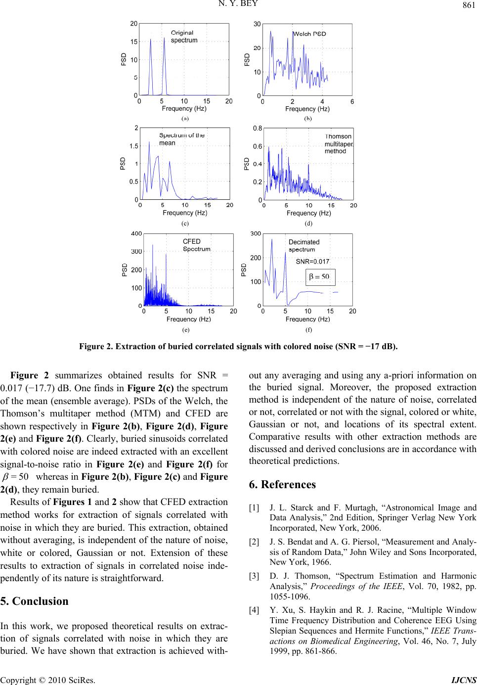

N. Y. BEY
861
Figure 2. Extraction of buried correlated signals with colored noise (SNR = −17 dB).
Figure 2 summarizes obtained results for SNR =
0.017 (−17.7) dB. One finds in Figure 2(c) the spectrum
of the mean (ensemble average). PSDs of the Welch, the
Thomson’s multitaper method (MTM) and CFED are
shown respectively in Figure 2(b), Figure 2(d), Figure
2(e) and Figure 2(f). Clearly, buried sinusoids correlated
with colored noise are indeed extracted with an excellent
signal-to-noise ratio in Figure 2(e) and Figure 2(f) for
50=

whereas in Figure 2(b), Figure 2(c) and Figure
2(d), they remain buried.
Results of Figures 1 and 2 show that CFED extraction
method works for extraction of signals correlated with
noise in which they are buried. This extraction, obtained
without averaging, is independent of the nature of noise,
white or colored, Gaussian or not. Extension of these
results to extraction of signals in correlated noise inde-
pendently of its nature is straightforward.
5. Conclusion
In this work, we proposed theoretical results on extrac-
tion of signals correlated with noise in which they are
buried. We have shown that extraction is achieved with-
out any averaging and using any a-priori information on
the buried signal. Moreover, the proposed extraction
method is independent of the nature of noise, correlated
or not, correlated or not with the signal, colored or white,
Gaussian or not, and locations of its spectral extent.
Comparative results with other extraction methods are
discussed and derived conclusions are in accordance with
theoretical predictions.
6. References
[1] J. L. Starck and F. Murtagh, “Astronomical Image and
Data Analysis,” 2nd Edition, Springer Verlag New York
Incorporated, New York, 2006.
[2] J. S. Bendat and A. G. Piersol, “Measurement and Analy-
sis of Random Data,” John Wiley and Sons Incorporated,
New York, 1966.
[3] D. J. Thomson, “Spectrum Estimation and Harmonic
Analysis,” Proceedings of the IEEE, Vol. 70, 1982, pp.
1055-1096.
[4] Y. Xu, S. Haykin and R. J. Racine, “Multiple Window
Time Frequency Distribution and Coherence EEG Using
Slepian Sequences and Hermite Functions,” IEEE Trans-
actions on Biomedical Engineering, Vol. 46, No. 7, July
1999, pp. 861-866.

862 N. Y. BEY
[5] N. Yahya Bey, “Extraction of Signals Buried in Noise,
Part I: Fundamentals,” Signal Processing, Vol. 86, No. 9,
September 2006, pp. 2464-2478.
[6] N. Yahya Bey, “Extraction of Signals Buried in Noise,
Part II: Experimental Results,” Signal Processing, Vol.
86, No. 10, 2006, pp. 2994-3011.
[7] N. A. Whitmal, J. C. Rutledge and J. Cohen, “Reducing
Correlated Noise in Digital Hearing Aids,” Engineering
in Medicine and Biology Magazine, IEEE Publication,
Vol. 15, No. 5, 1996, pp. 88-96.
[8] B. Goossens, A. Pizurica and W. Philips, “Removal of
Correlated Noise by Modeling Spatial Correlations and
Interscale Dependencies in the Complex Wavelet Do-
main,” IEEE International Conference on Image Proc-
essing, Ghent University, Ghent, Vol. 1, 2007, pp.
317-320.
[9] L. F. Villemoes, “Reduction of Correlated Noise Using a
Library of Orthonormal Bases,” IEEE Transactions on
Information Theory, Vol. 48, No. 2, February 2002, pp.
494-504.
[10] G. O. Karim, “Source Detection in Correlated Mul-
tichannel Signal and Noise Fields,” IEEE International
Conference on Acoustics, Speech and Signal Processing,
Vol. 5, 2003, pp. 257-60.
[11] V. Solo, “Signals in Coloured Noise: Joint
Non-Parametric Estimation of Signal and of Noise Spec-
trum,” IEEE International Conference on Acoustics,
Speech and Signal Processing, (ICASSP '03), Vol. 6,
April 2003, pp. 301-304.
[12] P. D. Welch, “The Use of Fast Fourier Transform for the
Estimation of Power Spectra: A Method Based on Time
Averaging over Short, Modified Periodograms,” IEEE
Transactions on Audio and Electroacoustics, Vol. 15, No.
2, January 1967, pp. 70-73.
[13] S. M. Kay and S. L. Marple, “Spectrum Analysis - A
Modern Perspective”, Proceedings of IEEE, Vol. 69, No.
11, November 1981, pp. 1380-1419.