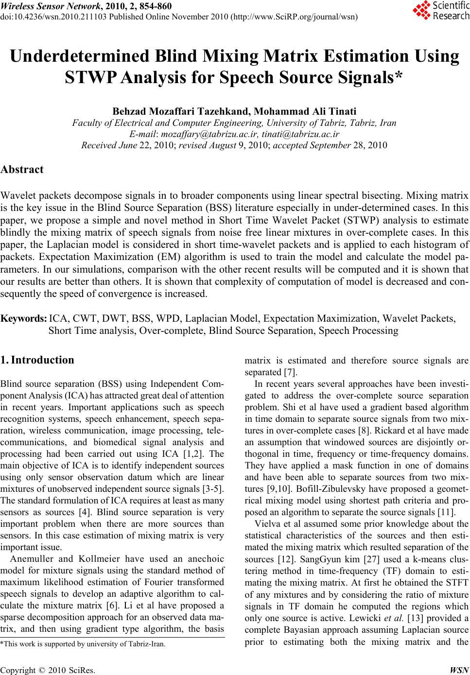Wireless Sensor Network, 2010, 2, 854-860
doi:10.4236/wsn.2010.211103 Published Online November 2010 (http://www.SciRP.org/journal/wsn)
Underdetermined Blind Mixing Matrix Estimation Using
STWP Analysis for Speech Source Signals*
Behzad Mozaffari Tazehkand, Mohammad Ali Tinati
Faculty of Electrical and Computer Engineering, University of Tabriz, Tabriz, Iran
Received June 22, 2010; revised August 9, 2010; accepted September 28, 2010
Abstract
Wavelet packets decompose signals in to broader components using linear spectral bisecting. Mixing matrix
is the key issue in the Blind Source Separation (BSS) literature especially in under-determined cases. In this
paper, we propose a simple and novel method in Short Time Wavelet Packet (STWP) analysis to estimate
blindly the mixing matrix of speech signals from noise free linear mixtures in over-complete cases. In this
paper, the Laplacian model is considered in short time-wavelet packets and is applied to each histogram of
packets. Expectation Maximization (EM) algorithm is used to train the model and calculate the model pa-
rameters. In our simulations, comparison with the other recent results will be computed and it is shown that
our results are better than others. It is shown that complexity of computation of model is decreased and con-
sequently the speed of convergence is increased.
Keywords: ICA, CWT, DWT, BSS, WPD, Laplacian Model, Expectation Maximization, Wavelet Packets,
Short Time analysis, Over-complete, Blind Source Separation, Speech Processing
1. Introduction
Blind source separation (BSS) using Independent Com-
ponent Analysis (ICA) has attracted great deal of attention
in recent years. Important applications such as speech
recognition systems, speech enhancement, speech sepa-
ration, wireless communication, image processing, tele-
communications, and biomedical signal analysis and
processing had been carried out using ICA [1,2]. The
main objective of ICA is to identify independent sources
using only sensor observation datum which are linear
mixtures of unobserved independent source signals [3-5].
The standard formulation of ICA requires at least as many
sensors as sources [4]. Blind source separation is very
important problem when there are more sources than
sensors. In this case estimation of mixing matrix is very
important issue.
Anemuller and Kollmeier have used an anechoic
model for mixture signals using the standard method of
maximum likelihood estimation of Fourier transformed
speech signals to develop an adaptive algorithm to cal-
culate the mixture matrix [6]. Li et al have proposed a
sparse decomposition approach for an observed data ma-
trix, and then using gradient type algorithm, the basis
matrix is estimated and therefore source signals are
separated [7].
In recent years several approaches have been investi-
gated to address the over-complete source separation
problem. Shi et al have used a gradient based algorithm
in time domain to separate source signals from two mix-
tures in over-complete cases [8]. Rickard et al have made
an assumption that windowed sources are disjointly or-
thogonal in time, frequency or time-frequency domains.
They have applied a mask function in one of domains
and have been able to separate sources from two mix-
tures [9,10]. Bofill-Zibulevsky have proposed a geomet-
rical mixing model using shortest path criteria and pro-
posed an algorithm to separate the source signals [11].
Vielva et al assumed some prior knowledge about the
statistical characteristics of the sources and then esti-
mated the mixing matrix which resulted separation of the
sources [12]. SangGyun kim [27] used a k-means clus-
tering method in time-frequency (TF) domain to esti-
mating the mixing matrix. At first he obtained the STFT
of any mixtures and by considering the ratio of mixture
signals in TF domain he computed the regions which
only one source is active. Lewicki et al. [13] provided a
complete Bayasian approach assuming Laplacian source
prior to estimating both the mixing matrix and the
*This work is supported by university of Tabriz-Iran.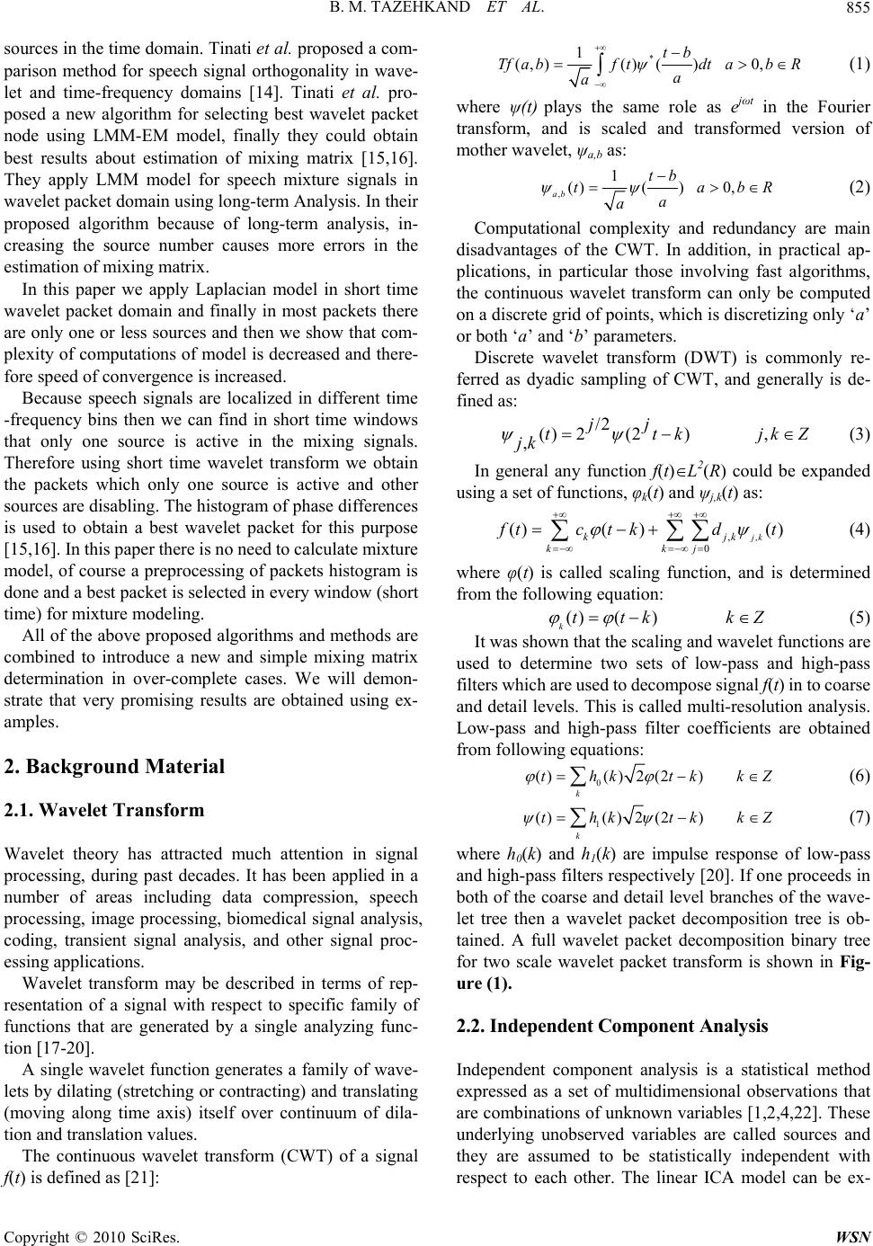

B. M. TAZEHKAND ET AL. 855
sources in the time domain. Tinati et al. proposed a com-
parison method for speech signal orthogonality in wave-
let and time-frequency domains [14]. Tinati et al. pro-
posed a new algorithm for selecting best wavelet packet
node using LMM-EM model, finally they could obtain
best results about estimation of mixing matrix [15,16].
They apply LMM model for speech mixture signals in
wavelet packet domain using long-term Analysis. In their
proposed algorithm because of long-term analysis, in-
creasing the source number causes more errors in the
estimation of mixing matrix.
In this paper we apply Laplacian model in short time
wavelet packet domain and finally in most packets there
are only one or less sources and then we show that com-
plexity of computations of model is decreased and there-
fore speed of convergence is increased.
Because speech signals are localized in different time
-frequency bins then we can find in short time windows
that only one source is active in the mixing signals.
Therefore using short time wavelet transform we obtain
the packets which only one source is active and other
sources are disabling. The histogram of phase differences
is used to obtain a best wavelet packet for this purpose
[15,16]. In this paper there is no need to calculate mixture
model, of course a preprocessing of packets histogram is
done and a best packet is selected in every window (short
time) for mixture modeling.
All of the above proposed algorithms and methods are
combined to introduce a new and simple mixing matrix
determination in over-complete cases. We will demon-
strate that very promising results are obtained using ex-
amples.
2. Background Material
2.1. Wavelet Transform
Wavelet theory has attracted much attention in signal
processing, during past decades. It has been applied in a
number of areas including data compression, speech
processing, image processing, biomedical signal analysis,
coding, transient signal analysis, and other signal proc-
essing applications.
Wavelet transform may be described in terms of rep-
resentation of a signal with respect to specific family of
functions that are generated by a single analyzing func-
tion [17-20].
A single wavelet function generates a family of wave-
lets by dilating (stretching or contracting) and translating
(moving along time axis) itself over continuum of dila-
tion and translation values.
The continuous wavelet transform (CWT) of a signal
f(t) is defined as [21]:
*
1
(,)()() 0,
tb
Tfa bftdtabR
a
a






 (1)
where ψ(t) plays the same role as ejωt in the Fourier
transform, and is scaled and transformed version of
mother wavelet, ψa,b as:
,
1
()() 0,
ab
tb
tabR
a
a



 (2)
Computational complexity and redundancy are main
disadvantages of the CWT. In addition, in practical ap-
plications, in particular those involving fast algorithms,
the continuous wavelet transform can only be computed
on a discrete grid of points, which is discretizing only ‘a’
or both ‘a’ and ‘b’ parameters.
Discrete wavelet transform (DWT) is commonly re-
ferred as dyadic sampling of CWT, and generally is de-
fined as:
/2
()2(2) ,
,
jj
ttkjkZ
jk



(3)
In general any function f(t)L2(R) could be expanded
using a set of functions, φk(t) and ψj,k(t) as:
,,
0
()()()
jkkjk
kkj
f
tctk dt 
 
 


(4)
where φ(t) is called scaling function, and is determined
from the following equation:
()()
kttk kZ



(5)
It was shown that the scaling and wavelet functions are
used to determine two sets of low-pass and high-pass
filters which are used to decompose signal f(t) in to coarse
and detail levels. This is called multi-resolution analysis.
Low-pass and high-pass filter coefficients are obtained
from following equations:
0
()()2(2)
k
thk tkkZ 


 (6)
1
()()2(2)
k
thk tkkZ 


 (7)
where h0(k) and h1(k) are impulse response of low-pass
and high-pass filters respectively [20]. If one proceeds in
both of the coarse and detail level branches of the wave-
let tree then a wavelet packet decomposition tree is ob-
tained. A full wavelet packet decomposition binary tree
for two scale wavelet packet transform is shown in Fig-
ure (1).
2.2. Independ ent C ompon ent A nal ysis
Independent component analysis is a statistical method
expressed as a set of multidimensional observations that
are combinations of unknown variables [1,2,4,22]. These
underlying unobserved variables are called sources and
they are assumed to be statistically independent with
respect to each other. The linear ICA model can be ex-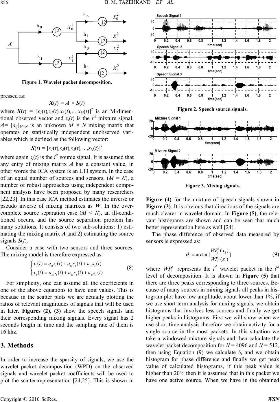

B. M. TAZEHKAND ET AL. 856
1
1
X
1
h
↓2
2
2
X
0
h
↓2
2
3
X
1
h
X
1
0
X
0
h
↓2
2
0
X
0
h
↓2
2
1
X
1
h
↓2
↓2
Figure 1. Wavelet packet decomposition.
pressed as: X(t) = A × S(t)
where X(t) = [x1(t),x2(t),x3(t),…,xM(t)]T is an M-dimen-
tional observed vector and xi(t) is the ith mixture signal.
A= [aij]M×N is an unknown M × N mixing matrix that
operates on statistically independent unobserved vari-
ables which is defined as the following vector:
S(t) = [s1(t),s2(t),s3(t),…,sN(t)]T
where again si(t) is the ith source signal. It is assumed that
any entry of mixing matrix A has a constant value, in
other words the ICA system is an LTI system. In the case
of an equal number of sources and sensors, (M = N), a
number of robust approaches using independent compo-
nent analysis have been proposed by many researchers
[22,23]. In this case ICA method estimates the inverse or
pseudo inverse of mixing matrixes as W. In the over-
complete source separation case (M < N), an ill-condi-
tioned occurs, and the source separation problem has
many solutions. It consists of two sub-solutions: 1) esti-
mating the mixing matrix A and 2) estimating the source
signals S(t).
Consider a case with two sensors and three sources.
The mixing model is therefore expressed as:
1111122133
2211222233
()()()()
()()() ()
x
tastastast
x
tastastast




 (8)
For simplicity, one can assume all the coefficients in
one of the above equations to have unit values. This is
because in the scatter plots we are actually plotting the
ratios of relevant magnitudes of signals that will be used
in later. Figures (2), (3) show the speech signals and
their corresponding mixing signals. Every signal has 2
seconds length in time and the sampling rate of them is
16 khz.
3. Methods
In order to increase the sparsity of signals, we use the
wavelet packet decomposition (WPD) on the observed
signals and wavelet packet coefficients will be used to
plot the scatter-representation [24,25]. This is shown in
00.2 0.4 0.6 0.811.2 1.4 1.6 1.8 2
-10
0
10
time(sec)
Speech Signal 1
00.2 0.4 0.6 0.811.2 1.4 1.6 1.8 2
-10
0
10
time(sec)
Spe e ch Signa l 2
00.2 0.4 0.6 0.811.2 1.4 1.6 1.8 2
-10
0
10
time(sec)
Speech Signal 3
Figure 2. Speech source signals.
00.2 0.4 0.6 0.8 11.2 1.4 1.6 1.8 2
-20
0
20
time(sec)
Mixture Signal 1
00.2 0.4 0.6 0.811.2 1.4 1.6 1.82
-20
0
20
time(sec)
Mixtur e Signal 2
Figure 3. Mixing signals.
Figure (4) for the mixture of speech signals shown in
Figure (3). It is obvious that directions of the signals are
much clearer in wavelet domain. In Figure (5), the rele-
vant histograms are shown and can be seen that much
better representation here as well [24].
The phase difference of observed data measured by
sensors is expressed as:
2
1
()
arctan[ ]
()
l
i
tl
i
WP x
WP x
  (9)
where l
i
WP represents the ith wavelet packet in the l
th
level of decomposition. It is shown in Figure (5) that
there are three peaks corresponding to three sources. Be-
cause of many sources in mixing signals all peaks in his-
togram plot have low amplitude, about lower than 1%, if
we use short term analysis for mixing signals, we obtain
histograms that involves less sources and finally we get
higher peaks in histograms. First we will show when we
use short time analysis therefore we obtain activity for a
single source in the most packets. In this situation we
take a windowed mixture signals and then calculate the
wavelet packet decomposition for N = 4096 and N = 512,
then using Equation (9) we calculate θt and we obtain
histogram for phase difference and finally we get peak
value of calculated histograms, if this peak value is
higher than 20% then it is assumed that in this packet we
have one active source. When we have in the obtained

B. M. TAZEHKAND ET AL. 857
-1.5 -1-0.5 00.5 11.
5
-2
-1
0
1
2
WP(X1)
WP(X2)
Figure 4. Scatter plot of x2(t) respect to x1(t) in wavelet
packet domain.
-2 -1.5 -1 -0.5 00.5 11.5 2
0
0.002
0.004
0.006
0.008
0.01
Angle(rad)
Histogram
Figure 5. Histogram of phase difference between wavelet
packets of x2(t), x1(t).
packets lower peaks in histograms then we can say that
there are many sources are active in this packet, it is
shown in Figures (6), (7). In Figure (6) it is shown that
when we select window length 4096, in all packets more
sources are active and their peak values is lower than
10% and with window length 512 many or all of the
packets contain only one source and peak value is higher
than 20%.
3.1. Selection of the Best Wavelet Packet Node in
Short Time Analysis
In this section we propose a new algorithm to select the
best node in wavelet packet domain for each source di-
rection, which are depicted in columns of the mixing
matrix. Considering mixtures of speech signals in the
time-frequency domain, it is more probable that each
speech signal be localized in different time-frequency
bins.
Therefore, we can state that there are packets where a
particular source may be localized better than the other
sources, when we apply short time analysis in wavelet
packet domain. Consequently dispersion of that particu-
lar source will be better and will show itself in much
higher amplitude and narrower width in the histogram
-2 -1012
0
2
4
6Histogram of packet1 (b)
-10 -505 10
-10
0
10 Scatter plot of packet1 (a)
-2 -1012
0
5
10
15 Histogram of packet2 (b)
-1 -0.500.5 1
-1
0
1Scatter plot of packet2 (a)
-1 -0.500.5 1
-2
0
2Scatter plot of packet3 (a)
-2 -1012
0
2
4
6Histogram of packet3 (b)
Figure 6. (a) Scatter plot of wavelet packets; (b) Histogram
of phase differences N = 4096.
-2 -1 0 1 2
0
10
20
30 Histogram of Packet1 (b)
-10 -50 5
-10
0
10 Scatter Plot of Packet1 (a)
-1 -0.5 00.5 11.5
-0.5
0
0.5
1Scatter Plot of Packet2 (a)
-2 -1 0 1 2
0
20
40
60 Histogram of Packet2 (b)
-5 05 10
-10
0
10 Scatter Plot of Packet3 (a)
-2 -1 0 1 2
0
20
40 Histogram of Packet3 (b)
Figure 7. (a) Scatter plot of wavelet packets; (b) Histogram
of phase differences N = 512.
plots than the other sources. This presumption leads us to
find a certain packet that will identify some sources bet-
ter than the others. In Figure (8) we describe a new
method based on short time analysis in wavelet packet
domain. According to the previous sections we choose a
window in time domain and then we calculate the phase
differences and then histogram is obtained if maximum
peak value is higher than 20% then it is suitable for cal-
culating Laplacian model about it, unless another win-
dow is chosen and this operation is repeated over the
mixing signals. Finally we sort peak values and corre-
sponding Laplacian parameters, then best parameters are
selected based on maximum peak value about any source
direction.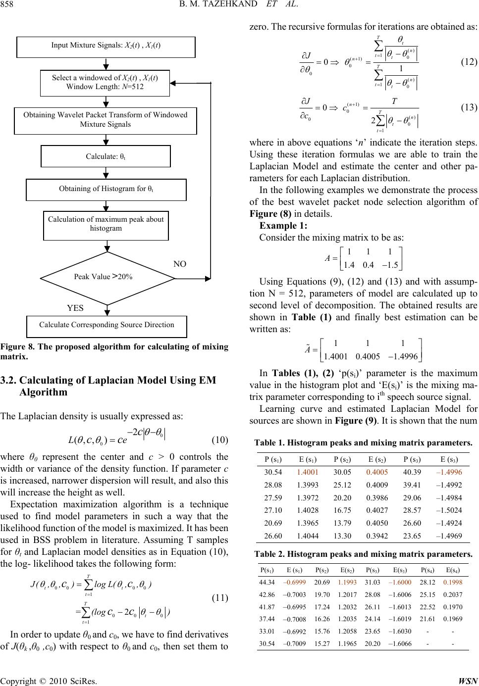

B. M. TAZEHKAND ET AL. 858
Figure 8. The proposed algorithm for calculating of mixing
matrix.
3.2. Calculating of Laplacian Model Using EM
Algorithm
The Laplacian density is usually expressed as:
0
0
2
(,, )Le
c
cc




 (10)
where θ0 represent the center and c > 0 controls the
width or variance of the density function. If parameter c
is increased, narrower dispersion will result, and also this
will increase the height as well.
Expectation maximization algorithm is a technique
used to find model parameters in such a way that the
likelihood function of the model is maximized. It has been
used in BSS problem in literature. Assuming T samples
for θt and Laplacian model densities as in Equation (10),
the log- likelihood takes the following form:
00 00
1
00 0
1
2
T
tt
t
T
t
t
J(,,)logL(,,)
=(log)
cc
cc
 








(11)
In order to update θ0 and c0, we have to find derivatives
of J(θk ,θ0 ,c0) with respect to θ0 and c0, then set them to
zero. The recursive formulas for iterations are obtained as:
()
10
(1)
0
0
()
10
0 1
T
t
n
tt
n
T
n
tt
J









 




(12)
(1)
0
()
0
0
1
0
2
n
T
n
t
t
JT
c
c






(13)
where in above equations ‘n’ indicate the iteration steps.
Using these iteration formulas we are able to train the
Laplacian Model and estimate the center and other pa-
rameters for each Laplacian distribution.
In the following examples we demonstrate the process
of the best wavelet packet node selection algorithm of
Figure (8) in details.
Example 1:
Consider the mixing matrix to be as:
11 1
1.4 0.41.5
A






Using Equations (9), (12) and (13) and with assump-
tion N = 512, parameters of model are calculated up to
second level of decomposition. The obtained results are
shown in Table (1) and finally best estimation can be
written as:
11 1
1.4001 0.40051.4996
A







In Tables (1), (2) ‘p(si)’ parameter is the maximum
value in the histogram plot and ‘E(si)’ is the mixing ma-
trix parameter corresponding to ith speech source signal.
Learning curve and estimated Laplacian Model for
sources are shown in Figure (9). It is shown that the num
Table 1. Histogram peaks and mixing matrix parameters.
P (s1)E (s
1) P (s2)E (s 2) P (s3) E (s3)
30.541.400130.050.4005 40.39 –1.4996
28.081.399325.120.4009 39.41 –1.4992
27.591.397220.200.3986 29.06 –1.4984
27.101.402816.750.4027 28.57 –1.5024
20.691.396513.790.4050 26.60 –1.4924
26.601.404413.300.3942 23.65 –1.4969
Table 2. Histogram peaks and mixing matrix parameters.
P(s1) E (s1) P(s2) E(s2) P(s3) E(s3) P(s4) E(s4)
44.34 –0.6999 20.69 1.1993 31.03 –1.6000 28.12 0.1998
42.86–0.7003 19.701.201728.08 –1.6006 25.150.2037
41.87–0.6995 17.241.203226.11 –1.6013 22.520.1970
37.44–0.7008 16.261.203524.14 –1.6019 21.610.1969
33.01–0.6992 15.761.205823.65 –1.6030 - -
30.54 –0.7009 15.271.196520.20 –1.6066 - -
Input Mixture Signals: X2(t) , X1(t)
Obtaining Wavelet Packet Transform of Windowed
Mixture Signals
Select a windowed of X2(t) , X1(t)
Window Length: N=512
Calculate: θt
Obtaining of Histogram for θt
Calculation of maximum peak about
histogram
NO
Peak Value >20%
YES
Calculate Corresponding Source Direction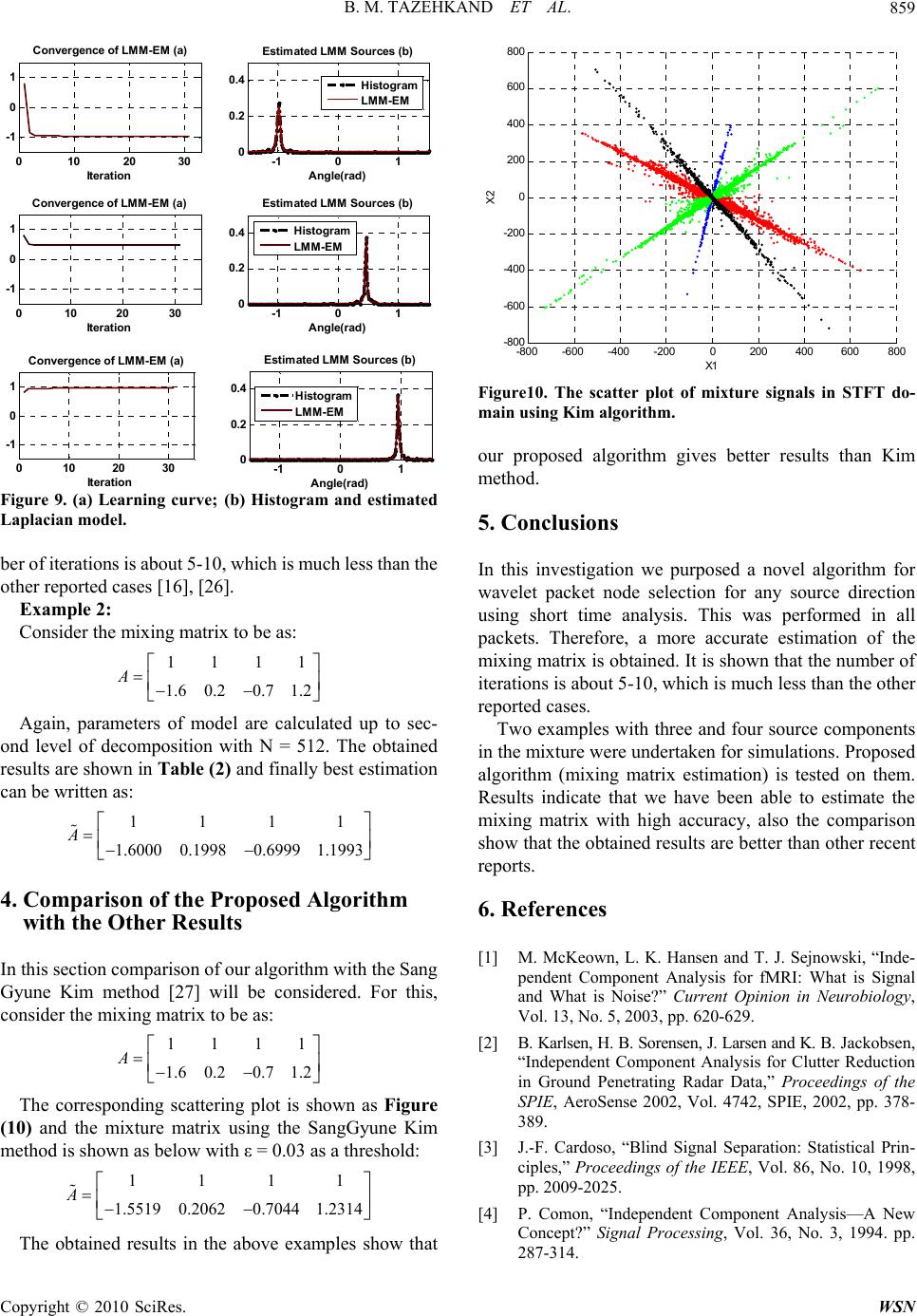

B. M. TAZEHKAND ET AL. 859
010 20 30
-1
0
1
Convergence of LMM-EM (a)
Iteration -1 0 1
0
0.2
0.4
Estimated LMM Sources (b)
Angle(rad)
Hi stog ram
LMM-EM
010 20 30
-1
0
1
Convergence of LMM-EM (a)
Iteration -1 0 1
0
0.2
0.4
Estimated LMM Sources (b)
Angle(rad)
Hi stog ram
LMM-EM
010 20 30
-1
0
1
Converge nc e of LMM-EM (a)
Iteration -1 01
0
0.2
0.4
Estimated LMM Sources (b)
An
g
le
(
rad
)
Histogram
LMM-EM
Figure 9. (a) Learning curve; (b) Histogram and estimated
Laplacian model.
ber of iterations is about 5-10, which is much less than the
other reported cases [16], [26].
Example 2:
Consider the mixing matrix to be as:
1111
1.60.20.7 1.2
A



Again, parameters of model are calculated up to sec-
ond level of decomposition with N = 512. The obtained
results are shown in Table (2) and finally best estimation
can be written as:
1111
1.60000.19980.69991.1993
A




4. Comparison of the Proposed Algorithm
with the Other Results
In this section comparison of our algorithm with the Sang
Gyune Kim method [27] will be considered. For this,
consider the mixing matrix to be as:
1111
1.60.20.7 1.2
A



The corresponding scattering plot is shown as Figure
(10) and the mixture matrix using the SangGyune Kim
method is shown as below with ε = 0.03 as a threshold:
1111
1.55190.20620.7044 1.2314
A




The obtained results in the above examples show that
-800 -600 -400 -2000200 400 600800
-800
-600
-400
-200
0
200
400
600
800
X1
X2
Figure10. The scatter plot of mixture signals in STFT do-
main using Kim algorithm.
our proposed algorithm gives better results than Kim
method.
5. Conclusions
In this investigation we purposed a novel algorithm for
wavelet packet node selection for any source direction
using short time analysis. This was performed in all
packets. Therefore, a more accurate estimation of the
mixing matrix is obtained. It is shown that the number of
iterations is about 5-10, which is much less than the other
reported cases.
Two examples with three and four source components
in the mixture were undertaken for simulations. Proposed
algorithm (mixing matrix estimation) is tested on them.
Results indicate that we have been able to estimate the
mixing matrix with high accuracy, also the comparison
show that the obtained results are better than other recent
reports.
6. References
[1] M. McKeown, L. K. Hansen and T. J. Sejnowski, “Inde-
pendent Component Analysis for fMRI: What is Signal
and What is Noise?” Current Opinion in Neurobiology,
Vol. 13, No. 5, 2003, pp. 620-629.
[2] B. Karlsen, H. B. Sorensen, J. Larsen and K. B. Jackobsen,
“Independent Component Analysis for Clutter Reduction
in Ground Penetrating Radar Data,” Proceedings of the
SPIE, AeroSense 2002, Vol. 4742, SPIE, 2002, pp. 378-
389.
[3] J.-F. Cardoso, “Blind Signal Separation: Statistical Prin-
ciples,” Proceedings of the IEEE, Vol. 86, No. 10, 1998,
pp. 2009-2025.
[4] P. Comon, “Independent Component Analysis—A New
Concept?” Signal Processing, Vol. 36, No. 3, 1994. pp.
287-314.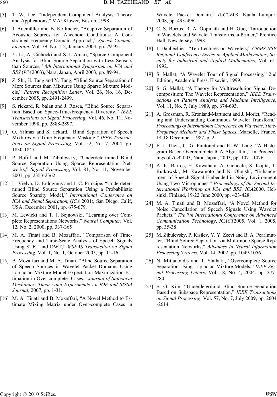

B. M. TAZEHKAND ET AL. 860
[5] T. W. Lee, “Independent Component Analysis: Theory
and Applications,” MA: Kluwer, Boston, 1998.
[6] J. Anemüller and B. Kollmeier, “Adaptive Separation of
Acoustic Sources for Anechoic Conditions: A Con-
strained Frequency Domain Approach,” Speech Commu-
nication, Vol. 39, No. 1-2, January 2003, pp. 79-95.
[7] Y. Li, A. Cichocki and S. I. Amari, “Sparce Component
Analysis for Blind Source Separation with Less Sensors
than Sources,” 4th International Symposium on ICA and
BSS (ICA2003), Nara, Japan, April 2003, pp. 89-94.
[8] Z. Shi, H. Tang and Y. Tang, “Blind Source Separation of
More Sources than Mixtures Using Sparse Mixture Mod-
els,” Pattern Recognition Letter, Vol. 26, No. 16, De-
cember 2005, pp. 2491-2499.
[9] S. rickard, R. balan and J. Rosca, “Blind Source Separa-
tion Based on Space-Time-Frequency Divercity,” IEEE
Transactions on Signal Processing, Vol. 46, No. 11, No-
vember 1998, pp. 2888-2897.
[10] O. Yilmaz and S. rickard, “Blind Separation of Speech
Mixtures via Time-Frequency Masking,” IEEE Transac-
tions on Signal Processing, Vol. 52, No. 7, 2004, pp.
1830-1847.
[11] P. Bofill and M. Zibulevsky, “Underdetermined Blind
Source Separation Using Sparce Representation Net-
works,” Signal Processing, Vol. 81, No. 11, November
2001, pp. 2353-2362.
[12] L. Vielva, D. Erdogmus and J. C. Principe, “Underdeter-
mined Blind Source Separation Using a Probabilistic
Source Sparsity Model,” International Conference on
ICA and Signal Separation, (ICA 2001), San Diego, Calif,
USA, December 2001, pp. 675-679.
[13] M. Lewicki and T. J. Sejnowski, “Learning over Com-
plete Representations Networks,” Neural Computer, Vol.
12, No. 2, 2000, pp. 337-365
[14] M. A. Tinati and B. Mozaffari, “Comparison of Time-
Frequency and Time-Scale Analysis of Speech Signals
Using STFT and DWT,” WSEAS Transaction on Signal
Processing, Vol. 1, No. 1, October 2005, pp. 11-16.
[15] B. Mozaffari and M. A. Tinati, “Blind Source Separation
of Speech Sources in Wavelet Packet Domains Using
Laplacian Mixture Model Expectation Maximization Es-
timation in Over-complete- Cases,” Journal of Statistical
Mechanics: Theory and Experiments An IOP and SISSA
Journal, 2007, pp. 1-31.
[16] M. A. Tinati and B. Mozaffari, “A Novel Method to Es-
timate Mixing Matrix under Over-complete Cases in
Wavelet Packet Domain,” ICCCE08, Kuala Lumpur,
2008, pp. 493-496.
[17] C. S. Burrus, R. A. Gopinath and H. Guo, “Introduction
to Wavelets and Wavelet Transforms, a Primer,” Prentice
Hall, New Jersey, 1998.
[18] I. Daubechies, “Ten Lectures on Wavelets,” CBMS-NSF
Regional Conference Series in Applied Mathematics, So-
ciety for Industrial and Applied Mathematics, Vol. 61,
1992.
[19] S. Mallat, “A Wavelet Tour of Signal Processing,” 2nd
Edition, Academic Press, Elsevier, 1999.
[20] S. G. Mallat, “A Theory for Multiresolution Signal De-
composition: The Wavelet Representation,” IEEE Trans-
actions on Pattern Analysis and Machine Intelligence,
Vol. 11, No. 7, July 1989, pp. 674-693.
[21] A. Grossman, R. Kronland-Martinent and J. Morlet, “Read-
ing and Understanding Continuous Wavelet Transform,”
Proceedings of International Conference on Wavelets, Time-
Frequency Methods and Phase Spaces, Marselle, France,
14-18 December, 1987, p. 2.
[22] F. J. Theis, C. G. Puntonet and E. W. Lang, “A Histo-
gram Based Overcomplete ICA Algorithm,” In Proceed-
ings of ICA2003, Nara, Japan, 2003, pp. 1071-1076.
[23] A. K. Barros, H. Kawahara, A. Cichocki, S. Kojita, T.
Rutkowski, M. Kawamoto and N. Ohnishi, “Enhance-
ment of Speech Signal Embedded in Noisy Environment
Using Two Microphones,” Proceedings of the Second In-
ternational Workshop on ICA and BSS, ICA2000, Hel-
sinki, Finland, 19-22 June 2000, pp. 423-428.
[24] M. A. Tinati and B. Mozaffari, “A Novel Method for
Noise Cancellation of Speech Signals Using Wavelet
Packets,” The 7th International Conference on Advanced
Communication Technology, ICACT2005, Vol. 1, 2005,
pp. 35-38
[25] M. Zibulevsky, P. Kisilev, Y. Y. Zeevi and B. A. Pearlmut-
ter, “Blind Source Separation via Multimode Sparse Rep-
resentation Networks,” Advances in Neural Information
Processing Systems, Vol. 14, 2002, pp. 1049-1056.
[26] N. Mitianoudis and T. Stathaki, “Overcomplete Source
Separation Using Laplacian Mixture Models,” IEEE Sig-
nal Processing Letters, Vol. 18, No. 4, 2004. pp. 277-
280.
[27] S. G. Kim, “Underdetermind Blind Source Separation
Based on Subspace Representation,” IEEE Transactions
on Signal Processing, Vol. 57, No. 7, July 2009, pp. 2604
-2614.