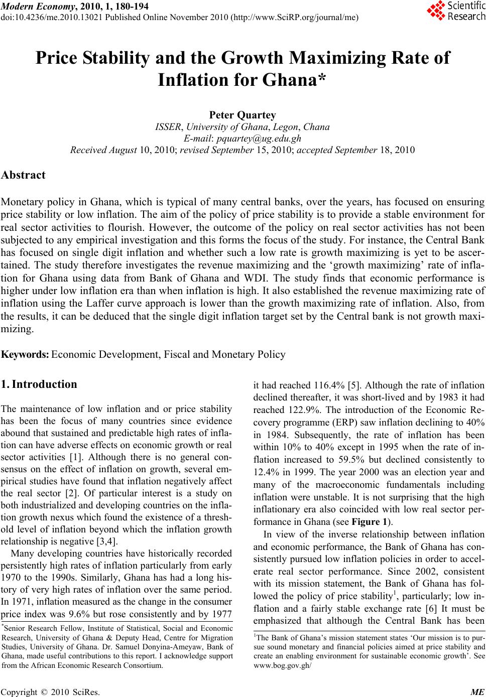Modern Economy, 2010, 1, 180-194
doi:10.4236/me.2010.13021 Published Online November 2010 (http://www.SciRP.org/journal/me)
Price Stability and the Growth Maximizing Rate of
Inflation for Ghana*
Peter Quartey
ISSER, University of Ghana, Legon, C hana
Received August 10, 2010; revised September 15, 2010; accept ed September 18, 2010
Abstract
Monetary policy in Ghana, which is typical of many central banks, over the years, has focused on ensuring
price stability or low inflation. The aim of the policy of price stability is to provide a stable environment for
real sector activities to flourish. However, the outcome of the policy on real sector activities has not been
subjected to any empirical investigation and this forms the focus of the study. For instance, the Central Bank
has focused on single digit inflation and whether such a low rate is growth maximizing is yet to be ascer-
tained. The study therefore investigates the revenue maximizing and the ‘growth maximizing’ rate of infla-
tion for Ghana using data from Bank of Ghana and WDI. The study finds that economic performance is
higher under low inflation era than when inflation is high. It also established the revenue maximizing rate of
inflation using the Laffer curve approach is lower than the growth maximizing rate of inflation. Also, from
the results, it can be deduced that the single digit inflation target set by the Central bank is not growth maxi-
mizing.
Keywords: Economic Development, Fiscal and Monetary Policy
1. Introduction
The maintenance of low inflation and or price stability
has been the focus of many countries since evidence
abound that sustained and predictable high rates of infla-
tion can have adverse effects on economic growth or real
sector activities [1]. Although there is no general con-
sensus on the effect of inflation on growth, several em-
pirical studies have found that inflation negatively affect
the real sector [2]. Of particular interest is a study on
both industrialized and developing countries on the infla-
tion growth nexus which found the existence of a thresh-
old level of inflation beyond which the inflation growth
relationship is negative [3,4].
Many developing countries have historically recorded
persistently high rates of inflation particularly from early
1970 to the 1990s. Similarly, Ghana has had a long his-
tory of very high rates of inflation over the same period.
In 1971, inflation measured as the change in the consumer
price index was 9.6% but rose consistently and by 1977
it had reached 116.4% [5]. Although the rate of inflation
declined thereafter, it was short-lived and by 1983 it had
reached 122.9%. The introduction of the Economic Re-
covery programme (ERP) saw inflation declining to 40%
in 1984. Subsequently, the rate of inflation has been
within 10% to 40% except in 1995 when the rate of in-
flation increased to 59.5% but declined consistently to
12.4% in 1999. The year 2000 was an election year and
many of the macroeconomic fundamentals including
inflation were unstable. It is not surprising that the high
inflationary era also coincided with low real sector per-
formance in Ghana (see Figure 1).
In view of the inverse relationship between inflation
and economic performance, the Bank of Ghana has con-
sistently pursued low inflation policies in order to accel-
erate real sector performance. Since 2002, consistent
with its mission statement, the Bank of Ghana has fol-
lowed the policy of price stability1, particularly; low in-
flation and a fairly stable exchange rate [6] It must be
emphasized that although the Central Bank has been
*Senior Research Fellow, Institute of Statistical, Social and Economic
Research, University of Ghana & Deputy Head, Centre for Migration
Studies, University of Ghana. Dr. Samuel Donyina-Ameyaw, Bank o
f
Ghana, made useful contributions to this report. I acknowledge suppor
t
from the African Economic Research Consortium.
1The Bank of Ghana’s mission statement states ‘Our mission is to pur-
sue sound monetary and financial policies aimed at price stability and
create an enabling environment for sustainable economic growth’. See
www.bog.gov.gh/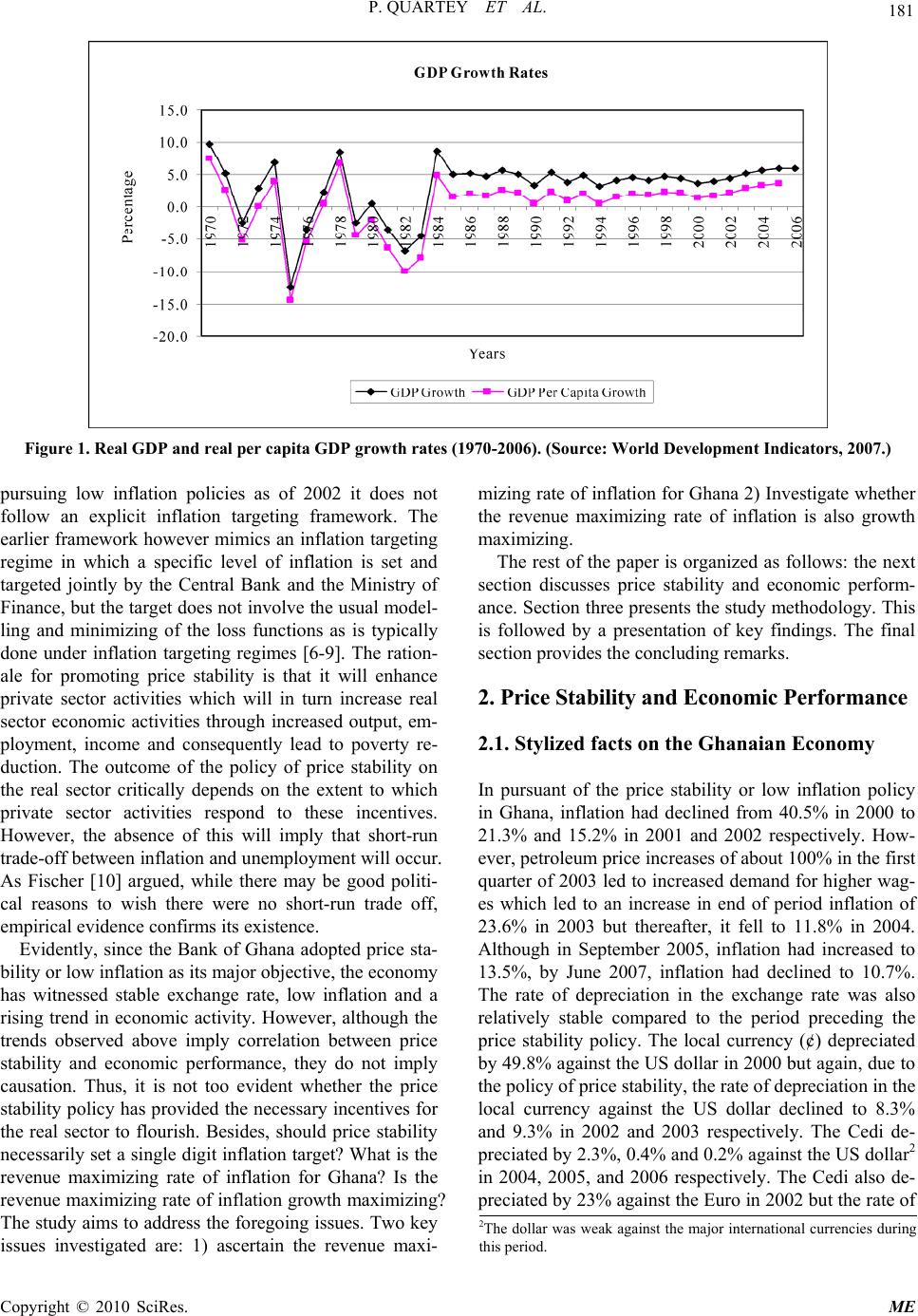

P. QUARTEY ET AL.
181
Figure 1. Real GDP and real per capita GDP growth rates (1970-2006). (Source: World Development Indicators, 2007.)
pursuing low inflation policies as of 2002 it does not
follow an explicit inflation targeting framework. The
earlier framework however mimics an inflation targeting
regime in which a specific level of inflation is set and
targeted jointly by the Central Bank and the Ministry of
Finance, but the target does not involve the usual model-
ling and minimizing of the loss functions as is typically
done under inflation targeting regimes [6-9]. The ration-
ale for promoting price stability is that it will enhance
private sector activities which will in turn increase real
sector economic activities through increased output, em-
ployment, income and consequently lead to poverty re-
duction. The outcome of the policy of price stability on
the real sector critically depends on the extent to which
private sector activities respond to these incentives.
However, the absence of this will imply that short-run
trade-off between inflation and unemployment will occur.
As Fischer [10] argued, while there may be good politi-
cal reasons to wish there were no short-run trade off,
empirical evidence confirms its existence.
Evidently, since the Bank of Ghana adopted price sta-
bility or low inflation as its major objective, the economy
has witnessed stable exchange rate, low inflation and a
rising trend in economic activity. However, although the
trends observed above imply correlation between price
stability and economic performance, they do not imply
causation. Thus, it is not too evident whether the price
stability policy has provided the necessary incentives for
the real sector to flourish. Besides, should price stability
necessarily set a single digit inflation target? What is the
revenue maximizing rate of inflation for Ghana? Is the
revenue maximizing rate of inflation growth maximizing?
The study aims to address the foregoing issues. Two key
issues investigated are: 1) ascertain the revenue maxi-
mizing rate of inflation for Ghana 2) Investigate whether
the revenue maximizing rate of inflation is also growth
maximizing.
The rest of the paper is organized as follows: the next
section discusses price stability and economic perform-
ance. Section three presents the study methodology. This
is followed by a presentation of key findings. The final
section provides the concluding remarks.
2. Price Stability and Economic Performance
2.1. Stylized facts on the Ghanaian Economy
In pursuant of the price stability or low inflation policy
in Ghana, inflation had declined from 40.5% in 2000 to
21.3% and 15.2% in 2001 and 2002 respectively. How-
ever, petroleum price increases of about 100% in the first
quarter of 2003 led to increased demand for higher wag-
es which led to an increase in end of period inflation of
23.6% in 2003 but thereafter, it fell to 11.8% in 2004.
Although in September 2005, inflation had increased to
13.5%, by June 2007, inflation had declined to 10.7%.
The rate of depreciation in the exchange rate was also
relatively stable compared to the period preceding the
price stability policy. The local currency (¢) depreciated
by 49.8% against the US dollar in 2000 but again, due to
the policy of price stability, the rate of depreciation in the
local currency against the US dollar declined to 8.3%
and 9.3% in 2002 and 2003 respectively. The Cedi de-
preciated by 2.3%, 0.4% and 0.2% against the US dollar2
in 2004, 2005, and 2006 respectively. The Cedi also de-
preciated by 23% against the Euro in 2002 but the rate of
2The dollar was weak against the major international currencies during
this period.

182 P. QUARTEY ET AL.
depreciation declined subsequently and by end 2006 it
had depreciated by 14.4% against the Euro. A similar
declining trend was observed for the British pound [5].
In terms of real sector performance, GDP and GDP
per capita growth rates demonstrate consistent and ap-
preciable increases during the period 2001-2006 (see
Table 1 & Figure 1).
It is also expected that under price stability, the lend-
ing rates will decline as inflation and the exchange rate
remains stable. This will increase access to credit by the
private sector which will in turn stimulate real sector
activity [11]. The average lending rate was 47% in 2000
but declined consistently thereafter and by end 2004, the
lending rate was 28.75% declining further to 27.75% by
September 2005. As of March 2007, lending rates ranged
from 15% to 33.5%. The decline in the prime rate and
the lending rate between 2001 and 2007 also led to mar-
ginal declines in the interest rate margins (Figure 2).
From the above, it is intuitively obvious that the key
macroeconomic fundamentals (especially inflation, ex-
change rate and the interest rate margin) have been stable
but whether this has translated into improved real sector
performance remains to be investigated.
2.2. The Inter-Relationship between Price
Stability and Real Sector Performance
Inflation leads to a reduction in future profitability of
investment, especially when inflation is associated with
price variability. It leads to conservative investment
strategies, slows investment and economic growth [12].
Inflation affects the international competitiveness of a
country by making exports more expensive which in turn
leads to balance of payments problems. However, al-
though the general consensus is that inflation negatively
impacts growth in the long-run, there have been studies
that have found the inflation-output-growth relationship
to be either positive or non-existent. Tobin [14], for ex-
ample, derives a positive effect of inflation on growth by
augmenting the classical model of growth to allow for
substitution between physical capital and money. His
theoretical framework suggests that an increase in the
inflation rate would cause economic agents to shift away
Table 1. Sectoral Growth Rates (1990-2006).
SECTORS
Period AgricultureIndustry Services All
1998 5.1 3.2 6.0 4.7
1999 3.9 4.9 5.0 4.4
2000 2.1 3.8 5.4 3.7
2001 4.0 2.9 5.1 4.2
2002 4.4 4.7 4.7 4.5
2003 6.1 5.1 4.7 5.2
2004 7.5 5.1 4.7 5.8
2005 6.5 5.6 5.4 5.8
2006 5.7 7.3 6.5 6.2
Averages
1990-94 1.1 4.1 7.0 4.3
1995-99 4.4 4.7 5.3 4.4
2000-06 5.2 4.9 5.2 5.1
Source: Computed from GoG Budget Statements, Several Issues.
Figure 2. Interest Rate Margins. The difference between the lending rate and the two rates (savings and time deposit rates).
Source: [13]) (

P. QUARTEY ET AL.
183
from holding money and to move towards more capital
investments, thereby increasing output. The money-in-
utility function model developed by Sidrauski [15], on
the other hand, finds that in the long run money is neutral
such that a rise in the rate of monetary expansion would
raise prices but leave the capital stock and output level
unaffected.
One of the early works that established a negative
long-run association between inflation and growth is that
of Stockman [16] who presented a cash-in-advance mod-
el of an economy in which money complemented capital.
Later work by Fischer [17] reinforced this negative rela-
tionship by stressing the role of macroeconomic uncer-
tainty in reducing the level of productivity and the rate of
investment. Rousseau and Wachtel [18] empirically ex-
plored the indirect role of financial sector development
in explaining the negative relationship between inflation
and growth. They argue that, a well developed and active
financial sector encourages a higher level of capital for-
mation and most importantly leads to improved alloca-
tion of capital.
In an inflationary environment, however, financial in-
termediaries would be reluctant to offer long-term fi-
nancing for capital formation and growth, and the vari-
ous measures (e.g. interest rate ceilings and credit alloca-
tion) instituted by government to protect certain sectors
of the economy would lead to inefficient allocations of
capital that inhibit growth. Other studies have also found
a negative link between inflation and growth. For in-
stance, Gillman et al. [19] studied 29 OECD and 18
APEC (Asia-Pacific Economic Cooperation) countries
from 1961 to 1997 and found a negative relationship
between inflation and economic performance. Similarly,
Barro [20] examined over 100 countries between the
years 1960 and 1990 and found a negative relationship
between inflation and growth.
Recent literature on the inflation-growth relationship
has been focused on the threshold effects of inflation on
growth. The possibility of this nonlinear effect of infla-
tion on growth was first examined by Fischer [17] who
found that the association between inflation and growth
weakens as inflation rises. The general view now, how-
ever, is that there exists a threshold level of inflation be-
low which the effect of inflation on growth is either posi-
tive or zero, and above which inflation has a negative
impact on growth. Bruno and Easterly [21-23], for ex-
ample, have cited evidence of a negative, short-to-me-
dium term relationship between high inflation (i.e. an
inflation rate of 40 percent or more) and growth, and no
evidence of a relationship between inflation and growth
at annual inflation rates less than 40 percent.
Khan and Senhadji [3] using a sample of 140 devel-
oping and industrial countries between 1960 and 1998
and also find evidence of the existence of a threshold
level of inflation beyond which the inflation-growth rela-
tionship is negative. Their findings also indicated that
this threshold level of inflation is higher for developing
countries (at 7-11 percent) than for industrialized ones
(1-3 percent). Similarly, Nell [4] study on the inflation-
ary episodes in South Africa (over the period 1960-1999)
also finds that single digit inflation may be beneficial to
growth while double digit inflation rates may be growth
retarding. Mariotti [2] using the Johansen Cointegration
approach found an inverse relationship between inflation
and economic growth. Similarly, Hodge [24] in examin-
ing the inflation-growth nexus for South Africa over the
period 1950-2002 confirmed the negative relationship
between inflation and growth over the medium to
long-run using the OLS method. He also adds that coun-
tries that maintain low inflation enjoy higher rates of
economic growth than countries with high rates of infla-
tion. It is important to add that ‘a certain amount of infla-
tion may help grease the wheels of the economy’ [25,26].
Thus, the evidence abounds from the above literature
that inflation negatively affects economic performance
and goes to confirm the existence of the threshold effect.
Unfortunately, these studies are mostly cross-country,
used simple OLS and have not been applied to Ghana
except in the case of [27,28] where the optimal rate of
inflation from 1970 to 1993 were estimated. It must be
noted that a lot has happened after this period and the
optimal rate of inflation as well as the inflation growth
nexus may have change and it is this gap in our knowl-
edge that this study intends to fill.
2.3 The Transmission Mechanism from Inflation
to Real Variables
The process through which changes in the monetary pol-
icy get transmitted to the ultimate objectives like infla-
tion or growth has come to be known as “monetary
transmission mechanism”. Interestingly, economists of-
ten refer to the channels of “monetary transmission” as a
black box–implying that we know that monetary policy
does influence output and inflation but we do not know
for certain how precisely it does so. Moreover, the im-
pact of inflation on real variables is not certain.
Nevertheless, in the literature, a number of transmis-
sion channels have been identified: (a) the quantum
channel (e.g., relating to money supply and credit); (b)
the interest rate channel; (c) the exchange rate channel;
and (d) the asset price channel. How these channels
function in a given economy depends on the stage of
development of the economy and its underlying financial
structure. Illustratively, in an open economy, one would
expect the exchange rate channel to be important; simi-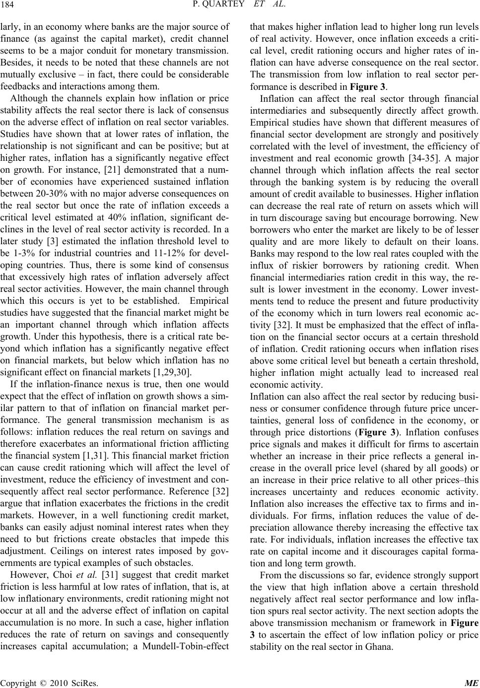

184 P. QUARTEY ET AL.
larly, in an economy where banks are the major source of
finance (as against the capital market), credit channel
seems to be a major conduit for monetary transmission.
Besides, it needs to be noted that these channels are not
mutually exclusive – in fact, there could be considerable
feedbacks and interactions among them.
Although the channels explain how inflation or price
stability affects the real sector there is lack of consensus
on the adverse effect of inflation on real sector variables.
Studies have shown that at lower rates of inflation, the
relationship is not significant and can be positive; but at
higher rates, inflation has a significantly negative effect
on growth. For instance, [21] demonstrated that a num-
ber of economies have experienced sustained inflation
between 20-30% with no major adverse consequences on
the real sector but once the rate of inflation exceeds a
critical level estimated at 40% inflation, significant de-
clines in the level of real sector activity is recorded. In a
later study [3] estimated the inflation threshold level to
be 1-3% for industrial countries and 11-12% for devel-
oping countries. Thus, there is some kind of consensus
that excessively high rates of inflation adversely affect
real sector activities. However, the main channel through
which this occurs is yet to be established. Empirical
studies have suggested that the financial market might be
an important channel through which inflation affects
growth. Under this hypothesis, there is a critical rate be-
yond which inflation has a significantly negative effect
on financial markets, but below which inflation has no
significant effect on financial markets [1,29,30].
If the inflation-finance nexus is true, then one would
expect that the effect of inflation on growth shows a sim-
ilar pattern to that of inflation on financial market per-
formance. The general transmission mechanism is as
follows: inflation reduces the real return on savings and
therefore exacerbates an informational friction afflicting
the financial system [1,31]. This financial market friction
can cause credit rationing which will affect the level of
investment, reduce the efficiency of investment and con-
sequently affect real sector performance. Reference [32]
argue that inflation exacerbates the frictions in the credit
markets. However, in a well functioning credit market,
banks can easily adjust nominal interest rates when they
need to but frictions create obstacles that impede this
adjustment. Ceilings on interest rates imposed by gov-
ernments are typical examples of such obstacles.
However, Choi et al. [31] suggest that credit market
friction is less harmful at low rates of inflation, that is, at
low inflationary environments, credit rationing might not
occur at all and the adverse effect of inflation on capital
accumulation is no more. In such a case, higher inflation
reduces the rate of return on savings and consequently
increases capital accumulation; a Mundell-Tobin-effect
that makes higher inflation lead to higher long run levels
of real activity. However, once inflation exceeds a criti-
cal level, credit rationing occurs and higher rates of in-
flation can have adverse consequence on the real sector.
The transmission from low inflation to real sector per-
formance is described in Figure 3.
Inflation can affect the real sector through financial
intermediaries and subsequently directly affect growth.
Empirical studies have shown that different measures of
financial sector development are strongly and positively
correlated with the level of investment, the efficiency of
investment and real economic growth [34-35]. A major
channel through which inflation affects the real sector
through the banking system is by reducing the overall
amount of credit available to businesses. Higher inflation
can decrease the real rate of return on assets which will
in turn discourage saving but encourage borrowing. New
borrowers who enter the market are likely to be of lesser
quality and are more likely to default on their loans.
Banks may respond to the low real rates coupled with the
influx of riskier borrowers by rationing credit. When
financial intermediaries ration credit in this way, the re-
sult is lower investment in the economy. Lower invest-
ments tend to reduce the present and future productivity
of the economy which in turn lowers real economic ac-
tivity [32]. It must be emphasized that the effect of infla-
tion on the financial sector occurs at a certain threshold
of inflation. Credit rationing occurs when inflation rises
above some critical level but beneath a certain threshold,
higher inflation might actually lead to increased real
economic activity.
Inflation can also affect the real sector by reducing busi-
ness or consumer confidence through future price uncer-
tainties, general loss of confidence in the economy, or
through price distortions (Figure 3). Inflation confuses
price signals and makes it difficult for firms to ascertain
whether an increase in their price reflects a general in-
crease in the overall price level (shared by all goods) or
an increase in their price relative to all other prices–this
increases uncertainty and reduces economic activity.
Inflation also increases the effective tax to firms and in-
dividuals. For firms, inflation reduces the value of de-
preciation allowance thereby increasing the effective tax
rate. For individuals, inflation increases the effective tax
rate on capital income and it discourages capital forma-
tion and long term growth.
From the discussions so far, evidence strongly support
the view that high inflation above a certain threshold
negatively affect real sector performance and low infla-
tion spurs real sector activity. The next section adopts the
above transmission mechanism or framework in Figure
3 to ascertain the effect of low inflation policy or price
stability on the real sector in Ghana.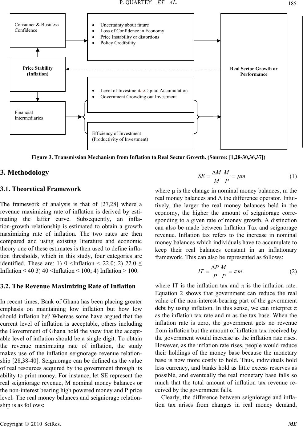

P. QUARTEY ET AL.
185
Consumer & Business
Confidence
Figure 3. Transmission Mechanism from Inflation to Real Sector Growth. (Source: [1,28-30,36,37])
3. Methodology
3.1. Theoretical Framework
The framework of analysis is that of [27,28] where a
revenue maximizing rate of inflation is derived by esti-
mating the laffer curve. Subsequently, an infla-
tion-growth relationship is estimated to obtain a growth
maximizing rate of inflation. The two rates are then
compared and using existing literature and economic
theory one of these estimates is then used to define infla-
tion thresholds, which in this study, four categories are
identified. These are: 1) 0 <Inflation < 22.0; 2) 22.0 ≤
Inflation ≤ 40 3) 40 <Inflation ≤ 100; 4) Inflation > 100.
3.2. The Revenue Maximizing Rate of Inflation
In recent times, Bank of Ghana has been placing greater
emphasis on maintaining low inflation but how low
should inflation be? Whereas some have argued that the
current level of inflation is acceptable, others including
the Government of Ghana hold the view that the accept-
able level of inflation should be a single digit. To obtain
the revenue maximizing rate of inflation, the study
makes use of the inflation seignorage revenue relation-
ship [28,38-40]. Seigniorage can be defined as the value
of real resources acquired by the government through its
ability to print money. For instance, let SE represent the
real seigniorage revenue, M nominal money balances or
the non-interest bearing high powered money and P price
level. The real money balances and seigniorage relation-
ship is as follows:
MM
SE m
M
P


 (1)
where μ is the change in nominal money balances, m the
real money balances and Δ the difference operator. Intui-
tively, the larger the real money balances held in the
economy, the higher the amount of seigniorage corre-
sponding to a given rate of money growth. A distinction
can also be made between Inflation Tax and seignorage
revenue. Inflation tax refers to the increase in nominal
money balances which individuals have to accumulate to
keep their real balances constant in an inflationary
framework. This can also be represented as follows:
PM
I
T
PP m


 (2)
where IT is the inflation tax and π is the inflation rate.
Equation 2 shows that government can reduce the real
value of the non-interest-bearing part of the government
debt by using inflation. In this sense, we can interpret π
as the inflation tax rate and m as the tax base. When the
inflation rate is zero, the government gets no revenue
from inflation but the amount of inflation tax received by
the government would increase as the inflation rate rises.
However, as the inflation rate rises, people would reduce
their holdings of the money base because the monetary
base is now more costly to hold. Thus, individuals hold
less currency, and banks hold as little excess reserves as
possible, and eventually the real monetary base falls so
much that the total amount of inflation tax revenue re-
ceived by the government falls.
Clearly, the difference between seigniorage and infla-
tion tax arises from changes in real money demand,
Financial
Intermediaries
 Level of Investment - Capital Accumulation
 Government Crowding out Investment
Efficiency of Investment
(Productivity of Investment)
Real Sector Growth or
Performance
 Uncertainty about future
 Loss of Confidence in Economy
 Price Instability or distortions
 Policy Credibility
Price Stability
(Inflation)

186 P. QUARTEY ET AL.
which in turn may be the consequence of financial liber-
alization or changes in the inflation rate, real income, and
interest rates. This difference is sometimes referred to as
the non-inflationary component of seigniorage, as it is
the increase in money demand that is consistent with a
zero inflation rate. As the economy grows the government
can obtain some revenue from seigniorage even if there is
no inflation. This is because as the demand for real money
grows, the government can create some base without pro-
ducing inflation. In the literature, a Laffer curve is usually
used to show how seigniorage revenue changes with the
inflation rate with an analogy to the conventional tax
revenues and tax rate. On the Laffer curve, there is a criti-
cal level of inflation at which the government can ‘maxi-
mize its seigniorage revenue’ and this critical level is
called the revenue maximizing inflation rate.
If the observed inflation rate is less than the estimated
seigniorage-maximizing inflation (optimal inflation rate)
the economy is said to be on the ‘correct side’ of the
Laffer curve and thus there is still opportunity for a
higher seigniorage at higher inflation rates. Also, there is
an implicit loss of seigniorage revenue if the economy
moves to a lower level of inflation. However, this might
have serious implications if the current inflation is per-
ceived to be less than the estimated critical level. Any
attempt to raise seigniorage revenue higher than the crit-
ical level by printing money may put the economy in a
higher inflationary path which could lead to hyperinfla-
tion. A typical Laffer curve is depicted below
Point S represents the seigniorage revenue as a pro-
portion of GDP and π the domestic inflation rate. In
Figure 4, it is evident that the seigniorage maximizing
inflation rate is B with a corresponding inflation rate of
π0. Below this point the higher the inflation rate the lar-
ger the seigniorage revenue by means of an increase in
the base money. However, to the right of the point B the
higher the domestic inflation the lower the seigniorage
revenue, since economic agents would try to avoid hold-
ing base money balances so as to protect them from in-
curring inflation tax. From Figure 4, it is evident that the
same seigniorage revenue can be collected by imposing
different inflation rates such as π2 and π1, where the tax
rate is higher but the tax base is lower, that is the wrong
side of the seigniorage maximizing Laffer curve in the
latter case with respect to the former. In this line, the
former coincides with the correct or efficient side of the
Laffer curve in which there is still opportunity for a
higher seigniorage at higher inflation rates and there is an
implicit loss of seigniorage revenue if the economy
moves to a lower level of inflation.
There have been a number of estimates of the magni-
tude of seigniorage revenue from both developed and de-
veloping economies. It is important, however, to distin-
Figure 4. The laffer curve.
guish between measures of pure inflation tax and meas-
ures of seigniorage revenue since only in the static steady
state will the two estimates be equivalent [28,41] pro-
vides two benchmark estimates of seigniorage and infla-
tion tax for a range of countries. He found that seign-
iorage usually accounts for approximately 0.5 percent of
GDP per annum. [28] also found that seignorage revenue
accounted for 2.5% of GDP in Ghana using quarterly
data from 1970 to 1993.
3.2.1. The Dynami c C ase–C oi ntegration Appr oach
At this stage, it is important to determine at what rate of
inflation will seigniorage revenue be maximized. Ac-
cording to [42], seigniorage revenue is maximized at the
rate of inflation at which the point elasticity of demand
for money is unity. This holds when the economy is in
the static steady state where the demand for real balances
is a function solely of inflation [28]. Implicitly, when the
economy is growing the revenue maximizing rate of in-
flation must lie below the optimal value. This is because
while the revenue from taxation of a given stock of real
balances is increasing in inflation, the real value of addi-
tional money balances held by agents in a growing
economy is monotonically decreasing in inflation. In
other words, π and M/P move in opposite directions.
In the quantity theory of money framework, govern-
ment can raise revenue without any inflationary pressure
by a parallel money growth to the rate of real growth.
Hence, an accompanying increase in the demand for real
money balances provides government with some ‘free’
resources. However, an excessive monetary growth be-
yond this real growth rate leads to inflation reducing the
purchasing power of the outstanding stock of real bal-
ances. This second phenomenon is the inflation tax, em-
phasizing this involuntary tax-like loss in the value of
money holdings although governments issue new cur-
rency through a set of voluntary transactions.
The inflation tax (IT) can be measured as

P. QUARTEY ET AL.
187
1.
PP
M
IT PP





(3)
The demand for real money balances takes a central
place in the study of seigniorage. However, other factors
apart from inflation explain the demand for money. In
the standard analysis the money demand is mainly a
function of inflation, and real income:

,
D
M
P






. (4)
Domestic and foreign assets substitution effects affect
the demand for money. Thus, the demand for money
function can be expressed in a homogenous logarithmic
form as
mymmb mr
Myb
P

r





 (5)
where M and P are the log of nominal money and prices
respectively, y is real income, П is the rate of inflation, b
is the rate of return on foreign assets (expected deprecia-
tion in the parallel exchange rate) and r is the domestic
interest rate (opportunity cost of domestic base money).
b and r have been expressed in the form of log (1 + x).
Re-arranging (5) and taking its time derivative gives the
growth in nominal money demand as
g
ggg
mymmbmr g
M
yb

  r
g
(6)
where, g denotes the growth rate (approximated by dlog
x/dt) of the variables. Substituting the above into (1), the
long run seignorage revenue expression is derived as
.
gggg
mymmb mr
SmM mybr

 

 

(7)
Assuming a money market equilibrium where Пg = 0
so that maximizing S with respect to П and rearranging
the first order conditions, a revenue maximizing value of
inflation rate is obtained as

*

g
g
mymb mr
mybr
m


 

g
t
(8)
The first term on the right represents the inverse of the
semi-elasticity of the demand for money with respect to
inflation since the demand for money function is the
semi-logarithm form in inflation. Cagan’s unit-elasticity
results is arrived at by imposing the restrictions yg = bg +
rg = 0. However, unit-elasticity only holds in the static
steady state. However, in general, the overall tax rate on
real balances is the sum of the inflation tax component
and the real money balances component. The revenue
maximizing rate of inflation will be affected by the rate
of income growth. Thus when income is growing, all
other things constant, the overall tax rate is above the
inflation rate. This occurs when inflation elasticity is
monotonically increasing in the inflation rate then the
rate at which revenue remains the same on the margin
must be less than the value which will yield unit elastic-
ity. Thus, once asset market effects are incorporated in
the demand for money function it becomes impossible to
ascertain analytically where it will lie but it is possible to
examine a number of stylized facts such as periods of
stagnation or stabilization and liberalization [28].
Using an econometric approach, the money demand
function above is estimated. Two key issues worth noting
are that the results are derived from the long run equilib-
rium demand for money function. Also, the possibility of
implicit weak exogeneity of the regressors of the condi-
tional model derived above is violated if inflation is en-
dogenous. To address these two issues, the [43,44] coin-
tegration method is employed.
The long-run money demand function can be refor-
mulated in a cointegrating system as follows:
11ttktk t
XXXD





  (9)
where X is a p x 1 non-stationary vector of variables,
namely, real money balances, real income, the domestic
interest rate, the premium on the parallel market rate and
the rate of inflation. Whereas μ contains the constants of
the system, D is a vector of centred seasonal dummies
while ε1 … εT are error terms which are assumed to be
independently normally distributed. The variables are
integrated of Order one and therefore a first difference
operator (∆) is applied. Subsequently, the equation in
first difference can be written as
11tt ktkkt
ktkt t
XXX X
XD  
1k



 
 

(10)
where Г1 = -(I-Пi - Пi) (i = 1…k-1), and П = -(I-Пi - Пi)
The above equation shows the stationary error-correction
first difference Vector Autogressive (VAR) framework
where the Г i∆Xt-k terms measure the short run dynamic
behaviour of the system while the ПiXt-k terms is the
long-run information (in levels) between the variables in
the VAR. ПiXt-k will be consistent with the stationary
VAR as long as it is also stationary and also the elements
of X are cointegrated. Thus, the number of cointegrated
vectors v between the elements of X will therefore de-
termine the rank of the vector П. П= -αβ’ where α and β
are v x p, with β containing the cointegrating vectors
while α measures the speed of adjustment from disequi-
librium or the feedback mechanism.
The next section will estimated the revenue maximiz-
ing rate of Inflation for Ghana from 1970 to 2006 using
the following data sources:
1) Domestic Money Bank Credit (1970-2006)-obtained
from WDI and ISSER SGER
2) GDP (1970-2006)–available from the World De-

P. QUARTEY ET AL.
188
velopment Indicators 2007
3) Lending and Deposit Rates (from 1970-2006)-ob-
tained from Bank of Ghana
4) Inflation (both monthly, quarterly and annual from
1970-2006) obtained from World Development Indica-
tors and/or Bank of Ghana
5) Business Confident Index (Available from June
2003 to June 2007). This is a bi-monthly data collected
by the Central on Business Perceptions about economic
progress
6) World Development Indicators (investment, popu-
lation growth, income per capita, secondary enrolment)
4. Findings
4.1. The Optimal Rate of Inflation
The evidence from the early 1990s to date is particularly
interesting; although inflation has declined, seigniorage
revenues have fallen further. Seigniorage revenues aver-
aged 0.9 per cent of GDP from 2001 to end 2006 with
inflation tax revenues averaging approximately 2.3 per
cent of GDP over the same period (i.e. 2001-2006). The
results are particularly striking because the liberalization
pursued to date has lowered transactions cost and in-
creased the opportunities for substitution between do-
mestic base money and foreign currency holding.
Tables 3 and 4 present the estimates of the unit root
test and the cointegrating system. The VAR is estimated
with a constant, seasonal dummy and six lags on each
variable (real income, real money balances, rate of infla-
tion, rate of return on foreign assets proxied by the ex-
pected depreciation of the parallel exchange rate and the
domestic interest rate) over the period 1990:1 to 2006:4.
The lag length was selected based on the SBC and the
Akaike Criteria. Unit root test were carried out on the
variables and those found to be non-stationary were dif-
ferenced (Table 2 and 3). The VAR was estimated em-
ploying the modified Cagan framework and the revenue
maximizing rate of inflation for Ghana is computed (See
Table 4). The results are robust and show that the reve-
nue maximizing rate of inflation for Ghana is 9.14 per
cent using quarterly data over the period 1990-2006. The
results also compares favourably with those of other
studies [28] where the revenue maximizing rate of infla-
tion between 1973 and 1990 was estimated to be around
15 per cent for Ghana. The study shows that the seign-
iorage maximising inflation rate for Ghana is below the
actual inflation rate, thus making the economy to lie on
the ‘wrong side’ of the Laffer curve. The current infla-
tion of 12.8 per cent is above the optimum level of 9.14
per cent. Another key issue yet to be addressed is
whether the revenue maximizing rate of inflation is also
the growth maximizing rate. This forms the focus of the
next section.
4.2. The Growth Maximizing Rate of
Inflation–Cointegrati on Appr oac h
To address the issue of whether the revenue maximizing
rate of inflation is also growth maximizing, a cointegra-
tion framework is used to analyze the inter-relationships
between growth and inflation. The approach is to build a
non-linear model which includes the squared term on
Table 2. Results of the unit root tests.
Augmented Dickey Fuller (ADF) Test Phillips Perron (PP) Test
VARIABLE Constant No Trend Constant Trend Constant No Trend Constant Trend
Rgdpg –1.826258 –1.687995 –3.774095 –2.410277
m/p 0.249605 –1.916955 0.852840 –2.979962
Deft –2.234099 –2.899822 –2.234099 –2.948491
Lexpt –2.010599 –1.842804 –1.864397 –.842804
Pvtinv –0.966095 –3.007251 –0.694917 –2.779045
Infl –2.183748 –2.559441 –2.425247 –2.56546
Test critical values:
1% level –3.540198 1% level –4.100935
5% level –2.909206 5% level –3.478305
10% level –2.592215 10% level –3.166788

P. QUARTEY ET AL.
189
Table 3. Cointegration tests.
Unrestricted Cointegration Rank Test (Trace)
Hypothesized No. of CE( s) Eigenvalue Trace Statistic 0.05 Critical Value Prob.**
None * 0.62755 85.12111 47.85613 0
At most 1 0.2557 24.87424 29.79707 0.1293
At most 2 0.103953 6.860256 15.49471 0.5257
At most 3 0.002697 0.164745 3.841466 0.6848
Unrestricted Cointegration Rank Test (Maximum Eigenvalue)
Hypothesized No. of CE(s) Eigenvalue Max-Eigen Statistic0.05 Critical Value Prob.**
None * 0.62755 60.24687 27.58434 0
At most 1 0.2557 18.01399 21.13162 0.1293
At most 2 0.103953 6.695511 14.2646 0.5257
At most 3 0.002697 0.164745 3.841466 0.6848
Trace test indicates 1 cointegrating eqn(s) at the 0.05 level; *denotes rejection of the hypothesis at the 0.05 level; **MacKinnon-Haug-Michelis
(1999) p-values.
Table 4. Cointegration results (dependent variable–real
money balances).
Variable Cointegration Equation
Y(–1) –0.9182 [–7.00446]
TB(–1) –0.06088 [–3.81129]
INF(–1) 0.117043 [6.97001]
C 1.611207
MP = -1.611207 + 0.918y + 0.06tb - 0.117inf; These results yield an opti-
mal inflation rate of (1/0.117 - 0.92*0.03) = 9.14%
inflation as an explanatory variable. Thus, the regression
equation is estimated as a second-degree polynomial.
This is a widely used technique for estimating non-linear
relationships by allowing for changes in slopes as a func-
tion of changes in the independent variable [27,28,45].
The squared inflation term is therefore used due to the
threshold effects. Hence, the slope of the estimated equa-
tion can vary with changes in the inflation rate. This en-
ables us to observe the turning point in the relationship
between inflation and growth.
The empirical model is specified as:
Real GDP Growth = β0 + β1(real balances) + β2(Exports/
GDP) + β3(Deficit/GDP) + β4(Private Investment/GDP) +
β5(Inflation) + β6(Human Capital) + β7(Inflation)2 β8
(Dummies) + ei
Three period dummies were introduced (1983-92;
1993-2000; and 2001-2006). These three periods mark
important economic regimes in Ghana. The list of vari-
ables and their definitions are provided in Appendix (Ta-
ble 5). Annual data from 1970-2006 were used and the
results are reported below. Both the ADF and the Phillips
Peron test confirm the existence of unit root in the vari-
ables. The I(1) variables were therefore differenced to
make them stationary and the results are presented in
Table 6 and 7.
The long run equation (equation 10) was estimated
using Johansen cointegration method and the results in-
dicate that there is one cointegrating vector and this is
confirmed by both the trace statistics and the Eigenval-
ues (Table 8). Subsequently, we test restrictions such as
unit elasticity. The vector error correction estimates of
the inflation growth relationship are presented in Table 6.
T abl e 5. Definition of vari ables.
Variable Definition
Rgdpg Real GDP Growth
m/p Real Balances
Deft Budget Deficit as a proportion of GDP
Lexpt Exports as a proportion of GDP
Pvtinv Private Investment as a share of GDP
Infl Inflation

P. QUARTEY ET AL.
190
Table 6. Results of the unit root tests.
Augmented Dickey Fuller (ADF) Test Phillips Perron (PP) Test
VARIABLE Constant No Trend Constant Trend Constant No Trend Constant Trend
Rgdpg –1.826258 –1.687995 –3.774095 –2.410277
m/p 0.249605 –1.916955 0.852840 –2.979962
Deft –2.234099 –2.899822 –2.234099 –2.948491
Lexpt –2.010599 –1.842804 –1.864397 –1.842804
Pvtinv –0.966095 –3.007251 –0.694917 –2.779045
Infl –2.183748 –2.559441 –2.425247 –2.56546
Test critical values:
1% level –3.540198 1% level –4.100935
5% level –2.909206 5% level –3.478305
10% level –2.592215 10% level –3.166788
Table 7. Results of the unit root tests (first difference).
Augmented Dickey Fuller (ADF) Test Phillips Perron (PP) Test
VARIABLE Constant No Trend Constant Trend Constant No Trend Constant Trend
dRgdpg –3.155835 –3.30395 –16.02544** –15.64752**
dm/p –10.056064** –10.090342** –11.35171** –11.92295**
dDeft –6.319811** –6.243196** –6.7806** –6.653737**
dlexpt –7.062333** –7.281371** –7.083831** –7.649226**
dPvtinv –7.677549** –6.478208** –8.439228** –16.62738**
dinfl –3.911792** –6.275686** –4.376691** –4.344887**
Test critical values:
1% level –4.110440 1% level –4.10320
5% level –3.482763 5% level –3.47937
10% level –3.169372 10% level –3.16740
GDP growth is negatively affected by inflation with a
one year lag. Private Investment has significantly posi-
tive effect on GDP growth. These findings corroborate
the work of [2,24]. From Table 9, the error correction
term or the speed of adjustment carries the right sign
(negative) and it is significant. The three period dummies
were insignificant except for the period 1983-1992 which
was weakly significant.
From Table 5, the turning point for the inflation-growth
relationship is calculated as follows:
Turning Point = -(Inflation Coefficient)/2*Inflation
Squared Coefficient). For the long run model, the turning
point or growth maximizing rate of inflation is 22.2%
while for the short run model, the growth maximizing
rate of inflation is 29.4%. From the above, it can be con-
cluded that the revenue ma imizing rate of inflation x

P. QUARTEY ET AL.
191
Table 8. Cointegrati o n tests.
Unrestricted Cointegration Rank Test (Trace)
Hypothesized No. of CE( s) Eigenvalue Trace Statistic 0.05 Critical Value Prob.**
None * 0.852706 132.8203 95.75366 0.0003
At most 1 0.530721 65.78386 69.81889 0.1006
At most 2 0.404756 39.30433 47.85613 0.2484
At most 3 0.269686 21.14692 29.79707 0.3486
At most 4 0.248448 10.14711 15.49471 0.2696
Unrestricted Cointegration Rank Test (Maximum Eigenvalue)
Hypothesized No. of CE(s) Eigenvalue Max-Eigen Statistic0.05 Cri tical Value Prob.**
None * 0.852706 67.03642 40.07757 0.2923
At most 1 0.530721 26.47953 33.87687 0.4821
At most 2 0.404756 18.15742 27.58434 0.6474
At most 3 0.269686 10.99981 21.13162 0.2121
At most 4 0.248448 9.996537 14.2646 0.2923
Trace test indicates 1 cointegrating eqn(s) at the 0.05 level; *denotes rejection of the hypothesis at the 0.05 level; **MacKinnon-Haug-Michelis
(1999) p-values.
(9.14%) is not growth maximizing but rather, the growth
maximizing rate of inflation is 22.2%. Thus, any infla-
tion rate above 22.2% will lead to moderate gains in
GDP growth. This corroborates the work of [45-48] who
found that for middle income countries, the inflation
threshold is 14-16 percent while for low income coun-
tries a range of 15-23 percent was obtained. For the en-
tire sample they consistently found that higher inflation
is associated with moderate gains in GDP growth up to
15-18 percent inflation threshold.
5. Conclusions and Policy Implications
The study investigates two key issues, namely, 1) ascer-
tain the revenue maximizing rate of inflation for Ghana 2)
Investigate whether the revenue maximizing rate of in-
flation is also growth maximizing. The analysis involved
estimating the revenue maximizing and growth maxi-
mizing rate of inflation. Thus, The Johansen cointegra-
tion approach was also used to analyze the effect of in-
flation on long term growth and found that inflation
negatively impacts on growth.
The study found that the economy had recorded very
high inflation rates during the pre-reform era and in 1982,
it was as high as 122.2%. However, after the reforms,
inflation rates have been lower and close to single digit.
Interestingly, the periods of high inflation were associ-
ated with lower growth rates (sometimes negative). GDP
growth rates have been positive since 1984 averaging
4.4% in 1995-99 and rising to 5.1% in 2000-2006. Ex-
cessively high rates of inflation affect real sector activi-
ties. The study found that the revenue maximizing rate of
inflation was 9.14 over the period 1990-2006. Thus, the
seignorage maximizing rate of inflation is below the in-
flation, indicating that the economy was operating on the
wrong side of the laffer curve. However, the revenue
maximizing inflation rate is not necessarily a growth
maximizing one. The growth maximizing rate of infla-
tion is 22.2%, thus corroborating observed historical
trends in growth and inflation rates in Ghana. Prior to the
economic reforms, Ghana had recorded significantly
high rates of inflation above the threshold and low (or
sometimes negative) growth rates. However, it recorded
significantly positive and high growth rates and low in-
flation during the post reform era.
In conclusion, price stability has led to higher growth
rates and the Ghanaian economy has operated below the
growth maximizing rate of inflation in recent times. It is
also obvious, that the growth maximizing rate of infla-
tion is not a single digit. Some level of inflation is cer-
tainly good for economic growth and job creation. The
study suggests that the government should pursue the

192 P. QUARTEY ET AL.
Table 9. Vector error correction estimates (Dependent variable–real GDP growth).
Variable Cointegration EquationVariable Error Correction Cointegration
Equation
EXPT(–1) –0.107658 [–1.6902] D(EXPT(–1)) 0.440554 [1.66582]
DEFT(–1) 0.261287 [1.85443] D(DEFT(–1)) –0.042573 [–0.10911]
INFL(–1) –0.083947 [–1.85164] D(DINFL(–1)) –0.037792 [–0.33322]
PVTINV(–1) –0.32954 [–1.97759] D(PVTINV(–1)) –0.671995 [–1.56096]
INFL SQD (–1) 0.001429 [3.85709] D(INFL SQD (–1)) 0.000851 [1.09857]
C 1.361557 C –0.850047 [–0.52506]
Dum1 3.494951 [1.45799]
Dum2 0.00236 [0.00094]
Dum3 1.362836 [0.47463]
EC Term –0.51846 [–1.72435]
R-Squared 0.50473
Adj. R-Squared 0.298367
Sum sq. resids 617.6098
S.E Equation 5.072844
F-statistic 2.445838
Log likelihood –99.89675
Akaike AIC 6.336957
Schwarz SC 6.825781
Mean Dependent 0.011429
S.D Dependent 6.056148
Log Likelihood –750.2182
Akaike Information Criterion46.9839
Schwarz Criterion 50.18347
price stability policy but also be mindful of the trade-off
between inflation and employment. Secondly, since the
growth maximizing rate of inflation for Ghana is not a
single digit, it is suggested that the government policy of
achieving single digit inflation should be considered
carefully taking into consideration inflation thresholds.
6. References
[1] J. H. Boyd, R. E. Levine and B. D. Smith, “The Impact of
Inflation on Financial Sector Performance,” Journal of
Monetary Econo m i cs, Vol. 47, No. 2, 2001, pp. 221-248.
[2] M. Mariotti, “An Examination of the Impact of Economic
Policy on Long-Run Economic Growth: An Application
of Vecm Structure to a Middle Income Context,” South
African Journal of Economics, Vol. 70, No. 4, 2002, pp.
689-724.
[3] M. S. Khan and A. S. Senhadji, “Threshold Effects in the
Relationship between Inflation and Growth,” IMF Staff
Papers, Vol. 48, No. 1, 2001, pp. 1-21
[4] K. Nell, “Is Low Inflation a Recondition for Faster

P. QUARTEY ET AL.
193
Growth? The Case of South Africa,” Working Paper No.
0011. Studies in Economics, University of Kent, Kent,
UK, 2000.
[5] Bank of Ghana, Statistical Bulletin, 2007.
[6] N. K. Sowa and P. Abradu-Otoo, “Inflation Management
in Ghana—The Output Factor,” Paper presented at the
Bank of England/Cornell University Workshop on New
Developments in Monetary Policy in Emerging Econo-
mies, London, 17-18 July 2007.
[7] J. Ammer and R. T. Freeman, “Inflation Targeting in the
1990s: The Experience of New Zealand, Canada and the
UK,” Journal of Economics and Business, Vol. 47, 1995,
pp. 165-192.
[8] N. Apergis, S. Miller, A. Panethimitakis and A. Vamva-
kidis, “Inflation Targeting and Output Growth: Evidence
from the European Union,” IMF Working Paper
WP/05/89, Washington DC, 2005.
[9] P. Arestis, G. M. Corporale and A. Cipollini, “Does In-
flation Targeting Affect the Trade-Off Between Output
Gap and Inflation Variability,” Manchester School, Vol.
70, No. 4, 2002, pp. 528-545.
[10] S. Fischer, “Maintaining Price Stability,” Finance and
Development, Vol. 33, No. 4. 1996, pp. 34-37.
[11] P. Quartey, “Finance and SME Development in Ghana,”
Journal of African Business, Vol. 4, No. 1, 2003, pp.
37-55.
[12] V. Gockal and S. Hanif, “Relationship between Inflation
and Economic Growth,” Working Paper No. WP2004/04.
Reserve Bank of Fiji, Fiji, 2004.
[13] ISSER State of Ghanaian Economy Report 2006, Univer-
sity of Ghana.
[14] J. Tobin, “Money and Economic Growth,” Econometrica,
Vol. 33, No. 4, 1965, pp. 671-684
[15] M. Sidrauski, “Rational Choice and Patterns of Growth in
a Monetary Economy,” The American Economic Review,
Vol. 57, No. 2, 1967, pp. 534-544.
[16] A. C. Stockman, “Anticipated Inflation and the Capital
Stock in a Cash-in-Advance Economy,” Journal of Mon-
etary Economics , Vol. 8, No. 3, 1981, pp. 387-393.
[17] S. Fischer, “The Role of Macroeconomic Factors in
Growth,” NBER Working Paper No. 4565, Cambridge,
Massachusetts, USA, 1993.
[18] P. L. Rousseau and P. Wachtel, “Inflation, Financial De-
velopment and Growth,” 2000. http://www.ssrn.com/ab-
stract=251589
[19] M. Gillman and K. Michal, “Modelling the Effect of In-
flation: Growth, Levels, and Tobin,” In: D. K. Levine, W.
Zame, L. Ausubel, P.-A Chiappori, B. Ellickson, A. Ru-
binstein and L. Samuelson, Eds., Proceedings of the 2002
North American Summer Meetings of the Econometric
Society: Money, 2002. http://www.dklevine.Com/ pro-
ceedings/money.htm
[20] R. J. Barro, “Inflation and Economic Growth,” NBER
Working Paper No. 5326, Cambridge, USA, 1995.
[21] M. Bruno and W. Easterly, “Inflation Crisis and Long-Run
Growth,” Journal of Monetary Economics, Vol. 41, No. 1,
1998, pp. 3-26.
[22] F. Breuss, “Was ECB’s Monetary Policy Optimal?” At-
lantic Economic Journal, Vol. 30, No. 3, 2002, pp.
298-321.
[23] S. Cocchetti and M. Ehrmann, “Does inflation increase
output volatility? An international comparison of policy-
makers’ preferences and outcomes,” Working Paper No.
69, Central Bank of Chile, Santiago, Chile, 2000.
[24] D. Hodge, “Inflation and Growth in South Africa,” Cam-
bridge Journal of Economics, Vol. 30, No. 2, 2006, pp.
163-180.
[25] G. A. Akerlof, W. Dickens and G. Perry, “The Macro-
economics of Low Inflation,” Brookings Papers on Eco-
nomic Activity, 1996, Vol. 1, pp. 1-59.
[26] G. A. Akerlof, W. Dickens and G. Perry, “Near-Rational
Wage and Price Setting and the Long-Run Phillips
Curve,” Brookings Papers on Economic Activity, 2000,
Vol. 1, pp. 1-60.
[27] N. K. Sowa, “Fiscal Deficits, Output and Inflation Tar-
gets in Ghana,” World Development, Vol. 22, No. 8, 1994,
pp. 1105-1117.
[28] C. Adam, B. Ndulu and N. K. Sowa, “Liberalization,
Seignorage Revenue in Kenya, Ghana and Tanzania,”
Journal of Development Studies, Vol. 34, No. 4, 1996, pp.
531-553.
[29] J. H. Boyd, R. E. Levine and B. D. Smith, “Capital Mar-
ket Imperfections in a Monetary Growth Model,” Eco-
nomic Theory, Vol. 11, No. 2, 1998, pp. 241-273
[30] E. Huybens and B. Smith, “Inflation, Financial Markets
and Long-Run Real Activity,” Journal of Monetary Eco-
nomics, Vol. 43, No. 2, 1998, pp. 283-315.
[31] S. Choi, B. Smith and J. H. Boyd, “Inflation, Financial
Markets and Capital Formation,” Federal Reserve Bank
of St. Louis Review, Vol. 78, 1996, pp. 41-58.
[32] J. H. Boyd and B. Champ, “Inflation, Banking and Eco-
nomic Growth,” Economic Commentary, Ohio, USA:
Federal Bank of Cleveland, 2006.
[33] R. G. King and R. Levine, “Finance, Entrepreneurship
and Growth: Theory and Evidence,” Journal of Monetary
Economics, Vol. 32, No. 3, 1993, pp. 513-542.
[34] R. Levine and S. Zervos, “Stock Markets, Banks and
Economic Growth,” American Economic Review, Vol. 88,
No. 3, 1998, pp. 537-558.
[35] Z. Xu, “Financial Development, Investment and Eco-
nomic Growth,” Economic Inquiry, Vol. 38, No. 2, 2000,
pp. 331-344.
[36] M. Li, “Inflation and Economic Growth: Threshold Ef-
fects and Transmission Mechanisms,” CEA Working Pa-
per 0176, Department of Economics, University of Al-
berta, Canada, 2006.
[37] E. Huybens and B. Smith, “Financial Market Frictions,
Monetary Policy and Capital Accumulation in a Small
Open Economy,” Journal of Economic Theory, Vol. 81,
No. 2, 1999, pp. 353-400.
[38] G. Khan and K. Parish, “Conducting Monetary Policy
with Inflation Targets,” Federal Reserve Bank of Kansas

P. QUARTEY ET AL.
194
City Economic Review, Vol. 83, 1998, pp. 5-32.
[39] M. King, 1997. “Changes in UK Monetary Policy: Rules
and Discretion in Practice,” Journal of Monetary Eco-
nomics, Vol. 39, No. 1, 1997, pp. 81-97.
[40] F. S. Mishkin and A. S. Posen, “Inflation Targeting: Les-
sons from Four African Countries,” Federal Reserve
Bank of New York Economic Policy Review, Vol. 3, No. 3,
1997, pp. 9-11
[41] S. Fischer, “Relative Price Variability and Inflation in the
United States and Germany,” European Economic Re-
view, Vol. 18, No. 2, 1982, pp. 171-196.
[42] P. Cagan, “The Monetary Dynamics of Hyper Inflation,”
In: M. Freedman, Ed., Studies in Quantity Theory of
Money, University of Chicago Press, Chicago, 1956, pp.
25-117.
[43] S. Johansen, “Statistical Analysis of Cointegrating Vec-
tors”. Journal of Economic Dynamics and Control, Vol.
12, No. 2-3, 1988, pp. 231-254.
[44] S. Johansen,“Domestic and Foreign Effects on Prices in
an Open Economy: The Case of Denmark,” Journal of
Policy Modelling, Vol. 14, No. 4, 1992, pp. 401-428.
[45] R. Pollin and A. Zhu 2005. “Inflation and economic
growth: A cross-country non-linear analysis,” Working
Paper Number 109, Political Economy Research Institute
Massachusetts, USA.
[46] L. E. O. Svensson, “Optimal Inflation Targets, Conserva-
tive Central Banks and Linear Inflation Contracts,”
American Economic Review, Vol. 87, No. 1, 1997, pp.
98-114.
[47] L. E. O. Svensson, “How Should Monetary Policy Be
Conducted in an Era of Price Stability? A Symposium
sponsored by the Federal Reserve Bank of Kansas City,”
New Challenges for Monetary Policy, 1999a, pp.
195-259.
[48] L. E. O. Svensson, “Inflation Targeting as a Monetary
Policy Rule,” Journal of Monetary Economics, Vol. 43,
No. 3, 1999b, pp. 607-654.