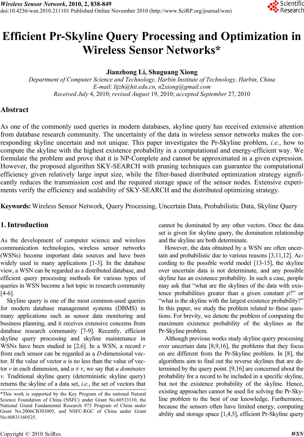Wireless Sensor Network, 2010, 2, 838-849
doi:10.4236/wsn.2010.211101 Published Online November 2010 (http://www.SciRP.org/journal/wsn)
Efficient Pr-Skyline Query Processing and Optimization in
Wireless Sensor Networks*
Jianzhong Li, Shuguang Xiong
Department of Computer Science and Technology, Harbin Institute of Technology, Harbin, China
Received July 4, 2010; revised August 19, 2010; accepted September 27, 2010
Abstract
As one of the commonly used queries in modern databases, skyline query has received extensive attention
from database research community. The uncertainty of the data in wireless sensor networks makes the cor-
responding skyline uncertain and not unique. This paper investigates the Pr-Skyline problem, i.e., how to
compute the skyline with the highest existence probability in a computational and energy-efficient way. We
formulate the problem and prove that it is NP-Complete and cannot be approximated in a given expression.
However, the proposed algorithm SKY-SEARCH with pruning techniques can guarantee the computational
efficiency given relatively large input size, while the filter-based distributed optimization strategy signifi-
cantly reduces the transmission cost and the required storage space of the sensor nodes. Extensive experi-
ments verify the efficiency and scalability of SKY-SEARCH and the distributed optimizing strategy.
Keywords: Wireless Sensor Network, Query Processing, Uncertain Data, Probabilistic Data, Skyline Query
1. Introduction
As the development of computer science and wireless
communication technologies, wireless sensor networks
(WSNs) become important data sources and have been
widely used in many applications [1-3]. In the database
view, a WSN can be regarded as a distributed database, and
efficient query processing methods for various types of
queries in WSN become a hot topic in research community
[4-6].
Skyline query is one of the most common-used queries
for modern database management systems (DBMS) in
many applications such as sensor data monitoring and
business planning, and it receives extensive concerns from
database research community [7-9]. Recently, efficient
skyline query processing and skyline maintenance in
WSNs have been studied in [2,6]. In a WSN, a record r
from each sensor can be regarded as a D-dimensional vec-
tor. If the value of vector u is no less than the value of vec-
tor v in each dimension, and u ≠ v, we say that u dominates
v. Traditional skyline query (deterministic skyline query)
returns the skyline of a data set, i.e., the set of vectors that
cannot be dominated by any other vectors. Once the data
set is given for skyline query, the domination relationship
and the skyline are both determinate.
However, the data obtained by a WSN are often uncer-
tain and probabilistic due to various reasons [3,11,12]. Ac-
cording to the possible world model [13-15], the skyline
over uncertain data is not determinate, and any possible
skyline has an existence probability. In such a case, people
may ask that “what are the skylines of the data with exis-
tence probabilities greater than a given constant p?” or
“what is the skyline with the largest existence probability?”
In this paper, we study the problem related to these ques-
tions. For brevity, we denote the problem of computing the
maximum existence probability of the skylines as the
Pr-Skyline problem.
Although previous works study skyline query processing
over uncertain data [8,9,16], the problems that they focus
on are different from the Pr-Skyline problem. In [8], the
algorithms aim to find out the reverse skylines that are de-
termined by the query point. [9,16] are concerned about the
probability for a record to be included in a specific skyline,
but not the existence probability of the skyline. Hence,
existing approaches cannot be used for solving the Pr-Sky-
line problem to the best of our knowledge. Furthermore,
because the sensors often have limited energy, computing
ability and storage space [1,4,5], efficient Pr-Skyline query
*This work is supported by the Key Program of the national Natural
Science Foundation of China (NSFC) under Grant No.60533110, the
N
ational Grand Fundamental Research 973 Program of China unde
r
Grant No.2006CB303005, and NSFC-RGC of China under Grant
N
o.60831160525.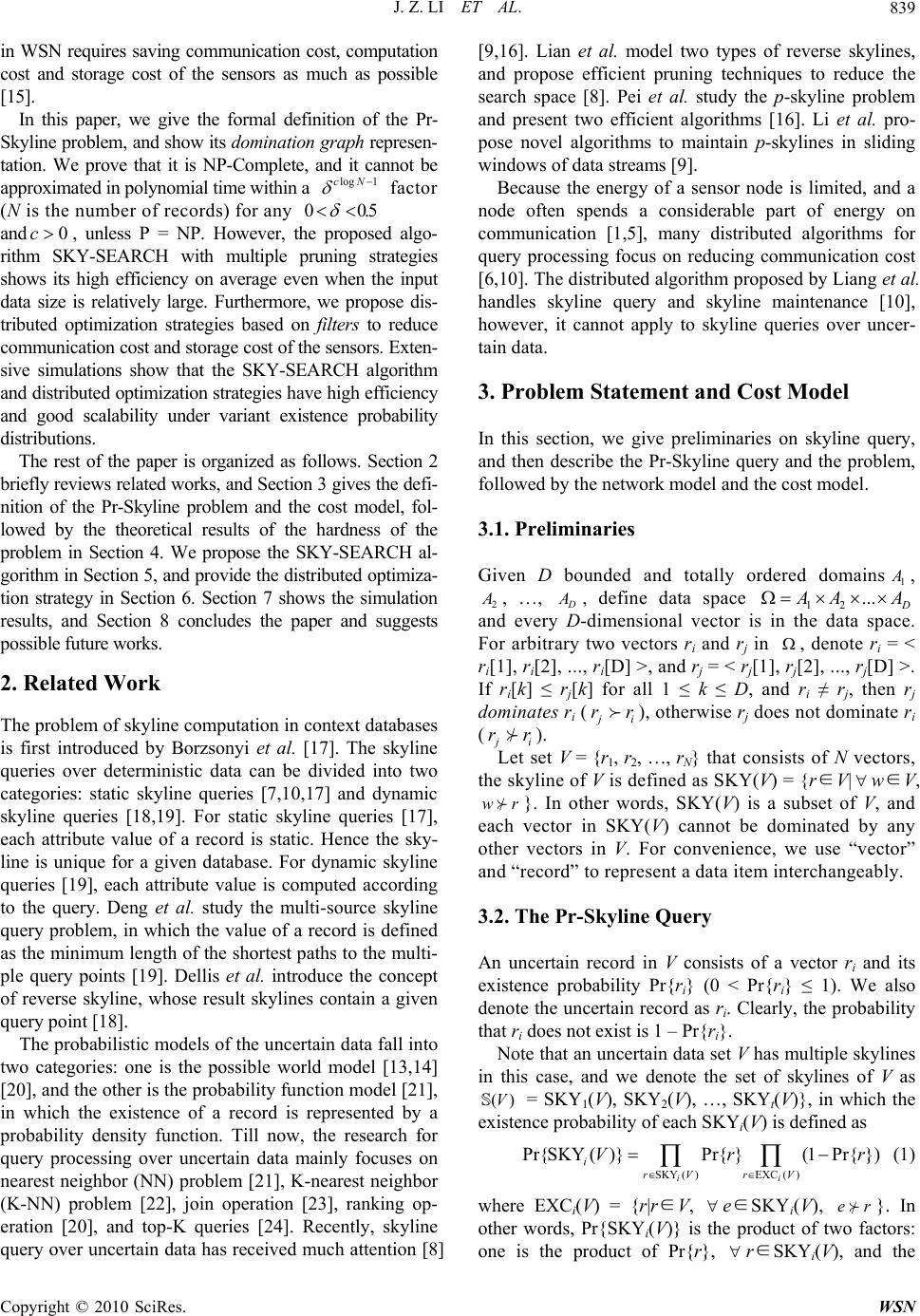

J. Z. LI ET AL. 839
in WSN requires saving communication cost, computation
cost and storage cost of the sensors as much as possible
[15].
In this paper, we give the formal definition of the Pr-
Skyline problem, and show its domination graph represen-
tation. We prove that it is NP-Complete, and it cannot be
approximated in polynomial time within a log 1cN 

factor
(N is the number of records) for any 0

0.5
and 0c, unless P = NP. However, the proposed algo-
rithm SKY-SEARCH with multiple pruning strategies
shows its high efficiency on average even when the input
data size is relatively large. Furthermore, we propose dis-
tributed optimization strategies based on filters to reduce
communication cost and storage cost of the sensors. Exten-
sive simulations show that the SKY-SEARCH algorithm
and distributed optimization strategies have high efficiency
and good scalability under variant existence probability
distributions.
The rest of the paper is organized as follows. Section 2
briefly reviews related works, and Section 3 gives the defi-
nition of the Pr-Skyline problem and the cost model, fol-
lowed by the theoretical results of the hardness of the
problem in Section 4. We propose the SKY-SEARCH al-
gorithm in Section 5, and provide the distributed optimiza-
tion strategy in Section 6. Section 7 shows the simulation
results, and Section 8 concludes the paper and suggests
possible future works.
2. Related Work
The problem of skyline computation in context databases
is first introduced by Borzsonyi et al. [17]. The skyline
queries over deterministic data can be divided into two
categories: static skyline queries [7,10,17] and dynamic
skyline queries [18,19]. For static skyline queries [17],
each attribute value of a record is static. Hence the sky-
line is unique for a given database. For dynamic skyline
queries [19], each attribute value is computed according
to the query. Deng et al. study the multi-source skyline
query problem, in which the value of a record is defined
as the minimum length of the shortest paths to the multi-
ple query points [19]. Dellis et al. introduce the concept
of reverse skyline, whose result skylines contain a given
query point [18].
The probabilistic models of the uncertain data fall into
two categories: one is the possible world model [13,14]
[20], and the other is the probability function model [21],
in which the existence of a record is represented by a
probability density function. Till now, the research for
query processing over uncertain data mainly focuses on
nearest neighbor (NN) problem [21], K-nearest neighbor
(K-NN) problem [22], join operation [23], ranking op-
eration [20], and top-K queries [24]. Recently, skyline
query over uncertain data has received much attention [8]
[9,16]. Lian et al. model two types of reverse skylines,
and propose efficient pruning techniques to reduce the
search space [8]. Pei et al. study the p-skyline problem
and present two efficient algorithms [16]. Li et al. pro-
pose novel algorithms to maintain p-skylines in sliding
windows of data streams [9].
Because the energy of a sensor node is limited, and a
node often spends a considerable part of energy on
communication [1,5], many distributed algorithms for
query processing focus on reducing communication cost
[6,10]. The distributed algorithm proposed by Liang et al.
handles skyline query and skyline maintenance [10],
however, it cannot apply to skyline queries over uncer-
tain data.
3. Problem Statement and Cost Model
In this section, we give preliminaries on skyline query,
and then describe the Pr-Skyline query and the problem,
followed by the network model and the cost model.
3.1. Preliminaries
Given D bounded and totally ordered domains1
A
,
2
A
, …,
D
A
, define data space 12 ...
D
A
AA 
and every D-dimensional vector is in the data space.
For arbitrary two vectors ri and rj in , denote ri = <
ri[1], ri[2], ..., ri[D] >, and rj = < rj[1], rj[2], ..., rj[D] >.
If ri[k] ≤ rj[k] for all 1 ≤ k ≤ D, and ri ≠ rj, then rj
dominates ri (
j
i
rr), otherwise rj does not dominate ri
(
j
i
rr

).
Let set V = {r1, r2, …, rN} that consists of N vectors,
the skyline of V is defined as SKY(V) = {r∈V|

w∈V,
wr

}. In other words, SKY(V) is a subset of V, and
each vector in SKY(V) cannot be dominated by any
other vectors in V. For convenience, we use “vector”
and “record” to represent a data item interchangeably.
3.2. The Pr-Skyline Query
An uncertain record in V consists of a vector ri and its
existence probability Pr{ri} (0 < Pr{ri} ≤ 1). We also
denote the uncertain record as ri. Clearly, the probability
that ri does not exist is 1 – Pr{ri}.
Note that an uncertain data set V has multiple skylines
in this case, and we denote the set of skylines of V as
()V = SKY1(V), SKY2(V), …, SKYt(V)}, in which the
existence probability of each SKYi(V) is defined as
SKY()EXC( )
Pr{SKY ()}Pr{}(1Pr{})
ii
irV rV
Vrr



 (1)
where EXCi(V) = {r|r∈V, e∈SKYi(V), er

}. In
other words, Pr{SKYi(V)} is the product of two factors:
one is the product of Pr{r}, r∈SKYi(V), and the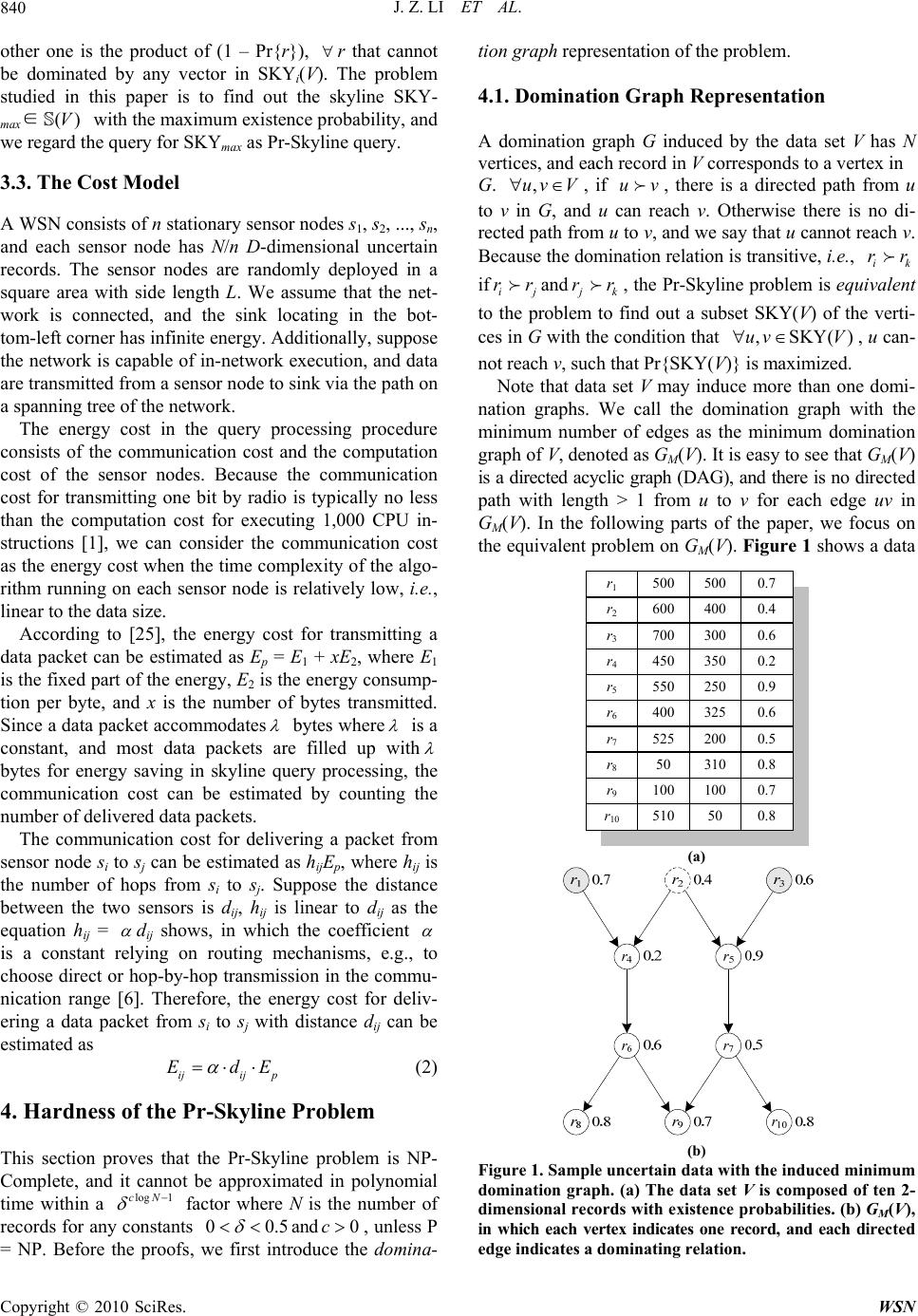

J. Z. LI ET AL. 840
other one is the product of (1 – Pr{r}), r that cannot
be dominated by any vector in SKYi(V). The problem
studied in this paper is to find out the skyline SKY-
max∈()V with the maximum existence probability, and
we regard the query for SKYmax as Pr-Skyline query.
3.3. The Cost Model
A WSN consists of n stationary sensor nodes s1, s2, ..., sn,
and each sensor node has N/n D-dimensional uncertain
records. The sensor nodes are randomly deployed in a
square area with side length L. We assume that the net-
work is connected, and the sink locating in the bot-
tom-left corner has infinite energy. Additionally, suppose
the network is capable of in-network execution, and data
are transmitted from a sensor node to sink via the path on
a spanning tree of the network.
The energy cost in the query processing procedure
consists of the communication cost and the computation
cost of the sensor nodes. Because the communication
cost for transmitting one bit by radio is typically no less
than the computation cost for executing 1,000 CPU in-
structions [1], we can consider the communication cost
as the energy cost when the time complexity of the algo-
rithm running on each sensor node is relatively low, i.e.,
linear to the data size.
According to [25], the energy cost for transmitting a
data packet can be estimated as Ep = E1 + xE2, where E1
is the fixed part of the energy, E2 is the energy consump-
tion per byte, and x is the number of bytes transmitted.
Since a data packet accommodates

bytes where

is a
constant, and most data packets are filled up with

bytes for energy saving in skyline query processing, the
communication cost can be estimated by counting the
number of delivered data packets.
The communication cost for delivering a packet from
sensor node si to sj can be estimated as hijEp, where hij is
the number of hops from si to sj. Suppose the distance
between the two sensors is dij, hij is linear to dij as the
equation hij =

dij shows, in which the coefficient

is a constant relying on routing mechanisms, e.g., to
choose direct or hop-by-hop transmission in the commu-
nication range [6]. Therefore, the energy cost for deliv-
ering a data packet from si to sj with distance dij can be
estimated as
ijij p
EdE

  (2)
4. Hardness of the Pr-Skyline Problem
This section proves that the Pr-Skyline problem is NP-
Complete, and it cannot be approximated in polynomial
time within a log 1cN 
 factor where N is the number of
records for any constants 00.5

 and 0c, unless P
= NP. Before the proofs, we first introduce the domin a-
tion graph representation of the problem.
4.1. Domination Graph Representation
A domination graph G induced by the data set V has N
vertices, and each record in V corresponds to a vertex in
G. ,uv V

, if uv, there is a directed path from u
to v in G, and u can reach v. Otherwise there is no di-
rected path from u to v, and we say that u cannot reach v.
Because the domination relation is transitive, i.e., ik rr
if ij rrand
j
k
rr, the Pr-Skyline problem is equivalent
to the problem to find out a subset SKY(V) of the verti-
ces in G with the condition that ,SKY()uv V , u can-
not reach v, such that Pr{SKY(V)} is maximized.
Note that data set V may induce more than one domi-
nation graphs. We call the domination graph with the
minimum number of edges as the minimum domination
graph of V, denoted as GM(V). It is easy to see that GM(V)
is a directed acyclic graph (DAG), and there is no directed
path with length > 1 from u to v for each edge uv in
GM(V). In the following parts of the paper, we focus on
the equivalent problem on GM(V). Figure 1 shows a data
500 5000.7r1
600 4000.4r2
700 3000.6r3
450 3500.2r4
550 2500.9r5
400 3250.6r6
525 2000.5r7
50310 0.8r8
100 1000.7r9
510 500.8r10
(a)
(b)
Figure 1. Sample uncertain data with the induced minimum
domination graph. (a) The data set V is composed of ten 2-
dimensional records with existence probabilities. (b) GM(V),
in which each vertex indicates one record, and each directed
edge indicates a dominating relation.

J. Z. LI ET AL. 841
set with 10 records and its minimum domination graph.
4.2. NP-Completeness
Now we prove that the decision format of the Pr-Sky-
line problem is NP-Complete, i.e., given data set V =
{r1, r2, ..., rN} and threshold T, to determine whether
there is a skyline SKY(V) of V, such that Pr{SKY(V)}
≥ T.
Theorem 1. The Pr-Skyline problem is NP-Com-
plete.
Proof: First, we can find out a skyline of V, and
compare its existence probability with T. Obviously,
the procedure can finish in polynomial time with re-
spect to N, which means that a solution to this problem
can be verified in polynomial time, and the Pr-Skyline
problem is in NP.
Then we construct a polynomial-time reduction
from the Minimum Set Cover (MSC) problem to the
Pr-Skyline problem. The MSC problem can be de-
scribed as: given set S, its m subsets, and integer K (K
≤ m), determine whether there are K of the given m
subsets, such that each item in S appears at least once
in the K subsets. For arbitrary instance of the MSC
problem, denote the n elements in S as e1, e2, …, en,
and denote the m subsets as S1, S2, …, Sm, we construct
an instance of the Pr-Skyline problem as follows. The
domination graph G has 1 (log 1)mnm







verti-
ces, in which m vertices refer to the m subsets of S,
and each 1 log 1m





vertices of the rest vertices
refers to an element in S. If
j
i
eS, we add a directed
edge from the vertex of Si to that of ej. Finally, let the
existence probability of each vertex be a constant
0.5

, and let (1 )
K
mK
T 

 . An example is il-
lustrated in Figure 2. Because the size of graph G is
polynomial with respect tomn

, the construction only
requires polynomial time.
If there are K subsets that cover all the elements in S
for the MSC problem, then these K vertices are se-
lected as the skyline of graph G. Because the K verti-











Figure 2. Construct an instance of Pr-Skyline from an in-
stance of MSC. Each ei refers to  
 1
log 1m

 vertices.
ces dominate all the vertices in ei (1 ≤ i ≤ n), and do
not dominate the rest m – K vertices, the existence prob-
ability of the skyline is (1 )
KmK
T 


. Hence this
skyline is a result to the Pr-Skyline problem.
Conversely, if there is a skyline SKY(V) such that
Pr{SKY(V)} ≥ T, then all the vertices in ei (1 ≤ i ≤ n)
are dominated by the vertices in SKY(V). To see this,
suppose that a vertex in some ei cannot be dominated
by the vertices in SKY(V), it is clear that all the verti-
ces in ei cannot be dominated by the vertices in
SKY(V). Let A = ei∩SKY(V) and B = ei\SKY(V), we
have Pr{SKY(V)} ≤Pr{}(1Pr{})
tA tB
tt



=
(1 )
tA tB





. Since 0.5


, Pr{SKY(V)} ≤
1
log 1
(1) m









<m

.
But Pr{SKY(V)} ≥ T =(1 )
K
mK


≥m

, a contradic-
tion. Therefore, all the vertices in ei (1 ≤ i ≤ n) are
dominated by the vertices in SKY(V). Suppose there
are x vertices of the subsets in the skyline, because
Pr{SKY(V)} =(1 )
x
mx


≥ T =(1 )
K
mK


 and,
0.5


, we have x ≤ K. Hence there must be K ≥ x
subsets covering all the elements in S.
Because the MSC problem is NP-Complete [26], the
Pr-Skyline problem is NP-Complete.
4.3. Property
Lemma 1 (Raz and Safra [27]). 0c

, the MSC
problem cannot be approximated within a lo gcN
factor
in polynomial time unless P = NP, in which N is the size
of the set to be covered.
Theorem 2. 00.5



,0c, the Pr-Skyline
problem cannot be approximated within a log 1cN


fac-
tor in polynomial time unless P = NP, in which N is the
number of data items.
Proof: Denote the qualities associated with an optimal
solution and an approximate solution for the MSC prob-
lem as OPT(MSC) and APP(MSC), respectively, and
denote those for the Pr-Skyline problem as OPT(P-SKY)
and APP(P-SKY), respectively. According to Lemma 2,
APP(MSC) ≥ clogN

OPT(MSC). Hence, approximation
algorithms for the instances of Pr-Skyline problem that
can be reduced from the MSC problem have the follow-
ing ratio bound.
APP(MSC) -APP(MSC)
OPT(MSC) -OPT(MSC)
log OPT(MSC)-log OPT(MSC)
OPT(MSC) -OPT(MSC)
(log 1)OPT(MSC)
APP(P-SKY)(1 )
OPT(P-SKY) (1 )
(1 )
(1 )
1
m
m
cN mcN
m
cN
















(3)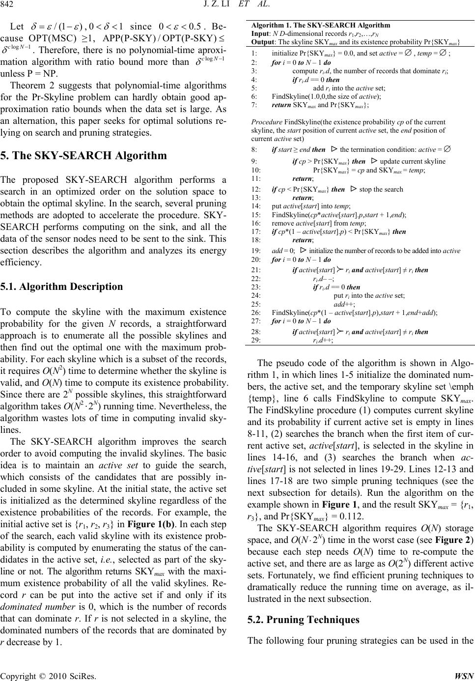

J. Z. LI ET AL. 842
Let /(1)

 ,01

 since 00.5

 . Be-
cause OPT(MSC) ≥1, APP(P-SKY) / OPT(P-SKY)

log 1cN

. Therefore, there is no polynomial-time aproxi-
mation algorithm with ratio bound more than log 1cN 

unless P = NP.
Theorem 2 suggests that polynomial-time algorithms
for the Pr-Skyline problem can hardly obtain good ap-
proximation ratio bounds when the data set is large. As
an alternation, this paper seeks for optimal solutions re-
lying on search and pruning strategies.
5. The SKY-SEARCH Algorithm
The proposed SKY-SEARCH algorithm performs a
search in an optimized order on the solution space to
obtain the optimal skyline. In the search, several pruning
methods are adopted to accelerate the procedure. SKY-
SEARCH performs computing on the sink, and all the
data of the sensor nodes need to be sent to the sink. This
section describes the algorithm and analyzes its energy
efficiency.
5.1. Algorithm Description
To compute the skyline with the maximum existence
probability for the given N records, a straightforward
approach is to enumerate all the possible skylines and
then find out the optimal one with the maximum prob-
ability. For each skyline which is a subset of the records,
it requires O(N2) time to determine whether the skyline is
valid, and O(N) time to compute its existence probability.
Since there are 2N possible skylines, this straightforward
algorithm takes O(N22N) running time. Nevertheless, the
algorithm wastes lots of time in computing invalid sky-
lines.
The SKY-SEARCH algorithm improves the search
order to avoid computing the invalid skylines. The basic
idea is to maintain an active set to guide the search,
which consists of the candidates that are possibly in-
cluded in some skyline. At the initial state, the active set
is initialized as the determined skyline regardless of the
existence probabilities of the records. For example, the
initial active set is {r1, r2, r3} in Figure 1(b). In each step
of the search, each valid skyline with its existence prob-
ability is computed by enumerating the status of the can-
didates in the active set, i.e., selected as part of the sky-
line or not. The algorithm returns SKYmax with the maxi-
mum existence probability of all the valid skylines. Re-
cord r can be put into the active set if and only if its
dominated number is 0, which is the number of records
that can dominate r. If r is not selected in a skyline, the
dominated numbers of the records that are dominated by
r decrease by 1.
Algorithm 1. The SKY-SEARCH Algorithm
Input: N D-dimensional records r1,r2,…,rN
Output: The skyline SKYmax and its existence probability Pr{SKYmax}
1: initialize Pr{SKYmax} = 0.0, and set active =, temp =

;
2: for i = 0 to N – 1 do
3: compute ri.d, the number of records that dominate ri;
4: if ri.d == 0 then
5: add ri into the active set;
6: FindSkyline(1.0,0,the size of active);
7: return SKYmax and Pr{SKYmax};
Procedure FindSkyline(the existence probability cp of the current
skyline, the start position of current active set, the end position of
current active set)
8: if start ≥ end then the termination condition: active =

9: if cp > Pr{SKYmax} then update current skyline
10: Pr{SKYmax} = cp and SKYmax = temp;
11: return;
12: if cp < Pr{SKYmax} then stop the search
13: return;
14: put active[start] into temp;
15: FindSkyline(cp*active[start].p,start + 1,end);
16: remove active[start] from temp;
17: if cp*(1 – active[start].p) < Pr{SKYmax} then
18: return;
19: add = 0; initialize the number of records to be added into active
20: for i = 0 to N – 1 do
21: if active[start]ri and active[start] ≠ ri then
22: ri.d– –;
23: if ri.d == 0 then
24: put ri into the active set;
25: add++;
26: FindSkyline(cp*(1 – active[start].p),start + 1,end+add);
27: for i = 0 to N – 1 do
28: if active[start]ri and active[start] ≠ ri then
29: ri.d++;
The pseudo code of the algorithm is shown in Algo-
rithm 1, in which lines 1-5 initialize the dominated num-
bers, the active set, and the temporary skyline set \emph
{temp}, line 6 calls FindSkyline to compute SKYmax.
The FindSkyline procedure (1) computes current skyline
and its probability if current active set is empty in lines
8-11, (2) searches the branch when the first item of cur-
rent active set, active[start], is selected in the skyline in
lines 14-16, and (3) searches the branch when ac-
tive[start] is not selected in lines 19-29. Lines 12-13 and
lines 17-18 are two simple pruning techniques (see the
next subsection for details). Run the algorithm on the
example shown in Figure 1, and the result SKYmax = {r1,
r3}, and Pr{SKYmax} = 0.112.
The SKY-SEARCH algorithm requires O(N) storage
space, and O(N

2N) time in the worst case (see Figure 2)
because each step needs O(N) time to re-compute the
active set, and there are as large as O(2N) different active
sets. Fortunately, we find efficient pruning techniques to
dramatically reduce the running time on average, as il-
lustrated in the next subsection.
5.2. Pruning Techniques
The following four pruning strategies can be used in the

J. Z. LI ET AL. 843
SKY-SEARCH algorithm.
Pruning strategy 1. Stop recursion if the existence
probability cp of the partially determined skyline in the
active set is less than current Pr{SKYmax}. This is be-
cause any skyline that contains the partially determined
part has its existence probability no more than cp, and
less than Pr{SKYmax}.
The rest three pruning strategies are based on the fol-
lowing three theorems, respectively.
Theorem 3. Denote I as the set of vertices that cannot
be dominated by any other vertices in domination graph
G, SKYmax {r|r ∈ I and Pr{r} > 0.5}.
Proof: Let R={r|r∈ I and Pr{ r} > 0.5}, according to
Equation (1),
SKY EXC
Pr{SKY}Pr{ }(1Pr{ })
max max
max rr
rr


 ,
in which EXCmax = {r|r∈V and e∈SKYmax, e
r}.
Suppose r, r∈R and rSKYmax. Let SKY’ = SKY-
max∪{r}, and EXC’ = {r|r∈V and e∈SKY’, e
r},
EXCmax = EXC’∪W∪{r}, in which
W = {e|e∈EXCmax\{r} and re}. Because r∈V, 0 <
Pr{r} ≤ 1, we have
SKY 'EXC '
SKY EXC
Pr{ }(1Pr{ })
Pr{SKY '}
Pr{SKY}Pr{ }(1Pr{ })
Pr{ }1
(1Pr{ })(1Pr{ })
max max
rr
max rr
eW
rr
rr
r
re










(4)
which means that there is a skyline SKY’ with
Pr{SKY’} > Pr{SKYmax}, a contradiction. Hence, r∈SKYmax
if r∈I and Pr{r} > 0.5.
Pruning strategy 2. If record u is dominated by a re-
cord in R = {r|r∈I, Pr{r} > 0.5}, then u cannot be in
SKYmax according to Theorem 3.
Theorem 4. If the domination graph G is composed of
k connected components G1, G2, ..., Gk, and there is no
edge between any two connected components, then
Pr{SKYmax} =
1
Pr{SKY( )}
k
i
i
G

.
Proof: Because there is no domination relation be-
tween any two connected components, the set SKY =
1
SKY( )
k
i
i
G

 is a skyline of G. Thus, Pr{SKYmax} ≥
1
Pr{SKY( )}
k
i
i
G

. Conversely, SKYmax∩Gi must be a
skyline of Gi for 1 ≤ i ≤ k, hence Pr{SKYmax} ≤
1
Pr{SKY( )}
k
i
i
G

. In summary, the equation holds.
Pruning strategy 3. Let Gu be the induced graph of
the records that are not in current temporary set (the
status of the records are not determined yet), compute the
connected components of Gu and the optimal solution for
each component, and then compute the global optimal
solution by Theorem 4. This divide-and-conquer strategy
avoids redundant computing of the domination relations,
and improves the performance of the algorithm.
Theorem 5. If the minimum domination graph G is a
directed tree, in which there is only one edge poin ting to
each vertex except the root of the tree, the Pr-Skyline
problem can be solved in polynomial time.
Proof: We prove this theorem by giving a polyno-
mial-time algorithm for this special case. Because the
tree root s cannot be dominated by any other vertices,
there are two cases for the skyline SKYmax: (1) s is in
SKYmax, and Pr{SKYmax} = Pr{s}. (2) s is not in SKYmax,
and Pr{SKYmax} = (1-Pr{s})
Child( )
OPT( )
rs
r
 according
to Theorem 4, where Child(s) is the children set of s, and
OPT(r) refers to the maximum existence probability of
the skylines in the tree rooted at vertex r. Because com-
puting OPT(r) is a sub-problem of the original problem,
it can be solved by dynamic programming as the follow-
ing equation:
Child( )
OPT()max{Pr{ },(1Pr{ })OPT()}
er
rrr e


 (5)
To obtain OPT(r), OPT(e) for e∈Child(r) should
be computed in advance. Hence the algorithm should run
in a bottom-up way, starting from the computation of the
leaves, and ending with OPT(s), which is Pr{SKYmax}.
For arbitrary vertex r in the tree, it requires O(|Child(r)|)
multiplies and O(1) comparisons to obtain OPT(r). Since
there are N vertices in the tree, the time complexity of
the algorithm is O(N

d), where d refers to the maximum
size of the children sets of the vertices. Furthermore, it
requires O(1) space to store OPT(r) r∈G, the space
complexity of the algorithm is O(N). Thus, we have pre-
sented a polynomial-time dynamic programming algo-
rithm, which completes the proof of the theorem.
Pruning strategy 4. Find out the forest that consists
of directed trees in the induced graph Gu, and compute
the skylines of the trees by the above dynamic program-
ming algorithm. If a directed tree is a single vertex r, the
skyline on the tree with maximum existence probability
max(P r{r}, 1 – Pr{r}) can be immediately computed
without enumerating the status of the vertex. Further-
more, this pruning strategy shows notable efficiency in
dealing with high-dimensional data because the domina-
tion graph is sparser than with low-dimensional data, and
there are probably more directed trees generated in the
search.
5.3. Energy Efficiency and Workload Balance
Energy efficiency. Consider the rectangle area on the
plane centered at (x, y) with the sink as the original point,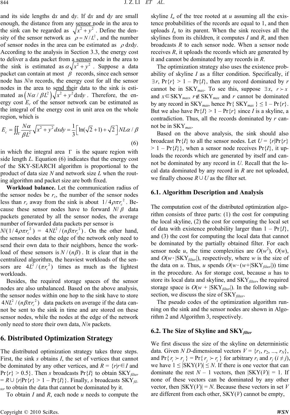

J. Z. LI ET AL. 844
and its side lengths dx and dy. If dx and dy are small
enough, the distance from any sensor node in the area to
the sink can be regarded as 22
x
y. Define the den-
sity of the sensor network as 2 /NL  , and the number
of sensor nodes in the area can be estimated as

dxdy.
According to the analysis in Section 3.3, the energy cost
to deliver a data packet from a sensor node in the area to
the sink is estimated as22
x
y  . Suppose a data
packet can contain at most

records, since each sensor
node has N/n records, the energy cost for all the sensor
nodes in the area to send their data to the sink is esti-
mated as

222
/ddNLxyxy  . Therefore, the en-
ergy cost Ec of the sensor network can be estimated as
the integral of the energy cost in unit area on the whole
region, which is
22
2
1ln( 21)2/
3
cN
Exydxdy NL
L







(6)
in which the integral area  is the square region with
side length L. Equation (6) indicates that the energy cost
of the SKY-SEARCH algorithm is proportional to the
product of data size N and network size L when the rout-
ing algorithm and packet size are both fixed.
Workload balance. Let the communication radius of
the sensor nodes be rc, the number of the sensor nodes
less than rc away from the sink is about 2 1/ 4c r

 . Be-
cause these sensor nodes have to forward N/

data
packets generated by all the sensor nodes, the average
number of forwarded data packets per sensor is
N/( 2
1/ 4c r

 ) = 22 4/( )
c
NLn r  . On the other hand,
the sensor nodes at the edge of the network only need to
send their own data to their neighbors, hence the work-
load of these sensors is/()Nn

. It is clear that in the
centralized algorithm, the heaviest workloads of the sen-
sors are 22 4/( )
c
Lr  times as much as the lightest
workloads.
Besides, the required storage spaces of the sensor
nodes are also unbalanced. Based on the above analysis,
the sensor nodes within one hop to the sink have to store
22
4/()
c
NLn r  data packets on average if the data can-
not be sent to the sink in time and are stored on these
sensor nodes, while the nodes at the edge of the network
only need to store their own data, N/n packets.
6. Distributed Optimization Strategy
The distributed optimization strategy takes three steps.
First, the sink s obtains I, the set of vertices that cannot
be dominated by any other vertices, and R = {r|r∈I and
Pr{r} > 0.5}. Then s broadcasts Pr{I} to obtain SKYfilter
= R∪{r|Pr{r} > 1 – Pr{I}}. Finally, s broadcasts SKYfil-
ter to obtain the data that cannot be dominated by it.
To obtain I and R, each node u needs to compute the
skyline Iu of the tree rooted at u assuming all the exis-
tence probabilities of the records are equal to 1, and then
uploads Iu to its parent. When the sink receives all the
skylines from its children, it computes I and R, and then
broadcasts R to each sensor node. When a sensor node
receives R, it uploads the records which are generated by
it and cannot be dominated by any records in R.
The optimization strategy also uses the existence prob-
ability of skyline I as a filter condition. Specifically, if

r, Pr{r} > 1 – Pr{I}, then any record dominated by r
cannot be in SKYmax. To see this, suppose

x, rx
and x∈SKYmax, r

SKYmax and r cannot be dominated
by any record in SKYmax, hence Pr{ SKYmax } ≤ 1 – Pr{r}.
But we also have Pr{I} > 1 – Pr{r} since I is a skyline, a
contradiction. Thus, all the records dominated by r can-
not be in SKYmax.
Based on the above analysis, the sink should also
broadcast Pr{I} to all the sensor nodes. Let U = {r|Pr{r}
> 1 – Pr{I}}, when a sensor node receives Pr{I}, it up-
loads the records which are generated by itself and can-
not be dominated by any record in U. Recall that the lo-
cal data dominated by any record in R are not uploaded,
we finally choose R∪U as the filter set.
6.1. Algorithm Description and Analysis
The computation cost of the distributed optimization algo-
rithm consists of three parts: (1) the cost for computing
the local skyline, (2) the cost for computing the local set
of data with existence probability larger than 1 – Pr{I},
and (3) the cost for computing the local data that cannot
be dominated by the partially obtained filter. For each
sensor node u, the time complexities are O(w2), O(w),
and O(w

|SKYfilter|), respectively, where w is the size of
the data on u. Thus, u spends O(w(w+|SKYfilter|)) time
in the procedure. As for storage cost, because u has to
store its local data and skyline, and SKYfilter, the required
storage space is O(w + |SKYfilter|). In the following sub-
section, we discuss the size of SKYfilter.
The pseudo codes of the optimization algorithm run-
ning on the sink and the sensor nodes are shown in Algo-
rithm 2 and Algorithm 3, respectively.
6.2. The Size of Skyline and SKYfilter
We first discuss the size of the skyline on deterministic
data. Given N D-dimensional vectors V = {r1, r2, ..., rN},
and Pr{ij rr} = Pr{
j
i
rr} for arbitrary ri and rj (i ≠ j),
we have 1 ≤ |SKY(V)| ≤ N. If there is one vector that can
dominate the rest N – 1 vectors, then |SKY(V)| = 1. If
none of these vectors can be dominated by any other
vector, then |SKY(V)| = N. Because these vectors in set V
are different from each other, SKY(V) cannot be empty,

J. Z. LI ET AL. 845
Algorithm 2. The optimization algorithm on the sink
1: broadcast the request for Pr-Skyline query;
2: receive the skylines from the children;
3: compute Pr{I} and R = {r|r∈I and Pr{r} > 0.5}, then broadcast
Pr{I};
4: receive the data from the children, and compute SKYfilter = R∪
U;
5: broadcast SKYfilter;
6: receive the filtered data from the children as the input of
SKY-SEARCH, and then compute SKYmax;
Algorithm 3. The optimization algorithm on the sensor nodes
1: receive and broadcast the request for Pr-Skyline query;
2: receive the skylines from the children;
3: compute local skyline and forward it to the parent;
4: receive and broadcast Pr{I} from the parent;
5: upload local records with existence probability larger than 1 –
Pr{I}, and forward the data from the children to the parent;
6: receive and broadcast SKYfilter;
7: upload local records not dominated by SKYfilter and forward the
data from the children to the parent;
i.e., |SKY(V)| ≠ 0.
Theorem 6. The expectation value of |SKY(V)| is

11
1
1
|()|1(1) (1)
Nii D
N
i
E
SKY VCiN




 


.
proof: First, we prove that Pr{ri∈SKY( V)} =
11
1
1
1(1) (1)
Nii D
N
i
Ci



 
. For arbitrary ri, rj∈V (i ≠ j),
because Pr{ri[k] ≥ rj[k]} = 2-1 for 1 ≤ k ≤ D, and the val-
ues in one dimension are independent from those in an-
other dimension, Pr{ij
rr} = 2-D. Generally, the prob-
ability for k vectors to simultaneously dominate ri is
Pr{rj1ri,rj2ri,...,rjk ri} =
D
k

.
If ri∈SKY(V), then ri cannot be dominated by the rest
N – 1 vectors. As a consequence, Pr{ri∈SKY(V)} = 1 –
Pr{r1ri OR ... OR ri-1 ri OR ri+1ri ... OR rNri}.
Because the events rjri and rkri (j, k ≠ i) are inde-
pendent, the equation can be rewritten as Pr{ri∈SK Y(V)}
= 1 – [1
1
N
CPr{ri is dominated by the rest 1 vector} –
2
1 N
CPr{ri is dominated by the rest 2 vectors} + ... +
1
1
(1)
NN
N
C

Pr{ri is dominated by the rest N – 1 vectors}]
=
11
1
1
1(1) (1)
Nii D
N
i
Ci



 
. Because there are N vectors,

11
1
1
|()|1(1)(1)
Nii D
N
i
ESKYVC iN




 



Theorem 6 indicates that the expected size of the sky-
line is far smaller than data size N, especially when D is
small. Figure 3 illustrates the expected size under dif-
ferent number of dimensions when N varies from 1 to 50.
Because R is the subset of some skyline on determi-
nistic data, the expected size of R cannot be larger than
|SKY(V)|. Moreover, the expected size of U is relative to
the existence probabilities of the data. If most existence
1020 3040 50
0
5
15
25
35
Number of data items
E(|skyline|)
D=6
D=4
D=2
Figure 3. The relation between the expected size of skyline
and the number of records with variant dimensions.
probabilities are near to 1, U may become very large.
Because SKYfilter = R∪U, the communication cost for
broadcasting SKYfilter is larger than that for collecting all
the data to the sink when U > N/n. In this case, it is a
better choice to let SKYfilter = R, regardless of U.
7. Simulations
The simulations consist of two parts: (1) the running time
of the SKY-SEARCH algorithm, and (2) the energy cost
of the distributed algorithm. The simulations run on ran-
domly-generated network topologies in a 300 by 300 m2
square area, and the communication radius varies from
50 m to 100 m. Each sensor node has 100 packets of data.
The existence probabilities of the records are of three
types: uniform distribution, normal distribution, and the
derived distribution from Poisson distribution. A record
in the derived distribution has an existence probability
/
x

where x is the value of the random variable in
Poisson distribution with1


, and

is the normaliza-
tion coefficient. In the derived distribution, most records
have existence probabilities near to 1. The simulations
run on a PC with a Pentium 2.0 GHz CPU and 2 GB
memory, and the network simulator is TOSSIM [28].
7.1. Running Time
When D = 2, the running time of the SKY-SEARCH
algorithm with variant data size is shown in Figure 4,
Figure 5 and Figure 6. When the number of records
varies from 10 to 105, the running time of the algorithm
without pruning (denoted as SKY-SEARCH in the fig-
ures) rapidly increases from 0ms to 104 ms level, while
the running time of the algorithm with pruning tech-
niques (denoted as SKY-SEARCH-OPT in the figures) is
of 1-2 orders of magnitude lower than the previous one.

J. Z. LI ET AL. 846
010100 100010000 100000
10
0
10
1
10
2
10
3
10
4
Number of data item s
Running time (ms)
SKY-SEARCH
SK Y- S EA RCH-OPT
Figure 4. Running time with uniform distribution of the
existence probabilities.
010 100100010000 100000
10
0
10
1
10
2
10
3
10
4
Number of data items
Running time (ms)
SKY- SEARCH
SKY- SEARCH-OPT
Figure 5. Running time with normal distribution of the
existence probabilities.
010100 100010000 100000
10
0
10
1
10
2
10
3
Numb er o f d ata ite ms
Running time (ms)
SKY-SEARCH
SKY-SEARCH-OPT
Figure 6. Running time with the derived distribution of the
existence probabilities.
010100100010000 100000
0
2
4
6
8
10
12
14
16
Number of data items
Skyline size
SKYmax
SKYfilter
Figure 7. Impact of D w ith uniform distribution of the exis-
tence probabilities.
010 100100010000 100000
0
2
4
6
8
10
12
14
16
Number of data items
S kyline size
SKYmax
SKYfilter
Figure 8. Impact of D with normal distribution of the exis-
tence probabilities.
010100100010000 100000
0
2
4
6
8
10
12
14
16
Numbe r of data i tems
Sk yline size
SKYmax
SKYfilter
Figure 9. Impact of D with the derived distribution of the
existence probabilities.

J. Z. LI ET AL. 847
When N = 200, the running time of the algorithm with
variant dimension D is illustrated in Figure 7, Figure 8,
and Figure 9. As D increases from 2 to 4, the algorithm
without pruning runs more than 108 ms (not shown in the
figures), while the algorithm with pruning runs less than
104 ms. Besides, the running time of the algorithm with
pruning appears to be a downward trend after rising for
the first. The reason is two-folds. First, when D begins to
increase from 2, the number of domination relations
starts to decrease from a very dense situation, hence the
search space increases. Second, when D increases to a
large number, i.e., 8, the number of domination relations
is fairly small, and pruning strategy 4 shows efficiency.
Figure 10, Figure 11 and Figure 12 depict the sizes of
SKYmax and SKYfilter with variant data size when D = 2.
The size of SKYmax grows from 2 to about 10 as the
number of records grows from 10 to 105. |SKYfilter| is
always larger than |SKYmax| with uniform distribution
2 4 6 810
10
0
10
1
10
2
10
3
10
4
Number of D
Running time (ms)
SKY-SEARCH
SK Y-S EA RCH- OPT
Figure 10. The sizes of SKYmax and SKYfilter with uniform
distribution of the existence prob.
2 4 6 810
10
0
10
1
10
2
10
3
10
4
Number of D
R
unn
i
ng
ti
me
(
ms
)
SKY-SEARCH
SKY-SEARCH-OPT
Figure 11. The sizes of SKYmax and SKYfilter with normal
distribution of the existence prob.
246810
10
0
10
1
10
2
10
3
10
4
Number of D
Ru nning tim e (ms)
SKY-SEARCH
SKY-SEARCH-OPT
Figure 12. The sizes of SKYmax and SKYfilter with the de-
rived distrib. of the existenc e prob.
and normal distribution, while they are almost the same
with the derived distribution. These results are consistent
with the analysis in Section 6.
7.2. Energy Cost
The workloads of the sensor nodes of a 100-node net-
work are illustrated in Figure 13, Figure 14, and Figure
15. The workloads of a sensor node u in both algorithms
are sorted by the number of packets sent by u without the
optimization in descending order. For all of the three
distributions, there are more than 20 nodes whose work-
loads are more than 100 packets, while all of the nodes
forward less than 100 packets with the optimization.
Figure 16 illustrates the energy cost of the network as
the network size grows from 20 nodes to 100 sensor
nodes. The number of packets grows from about 5000 to
more than 25000 when using the algorithm without op-
timization, and each node send more than 250 packets on
average. With the optimization, the number of packets
grows slowly (about 5000 packets when there are 100
sensor nodes). These results indicate that the optimiza-
tion strategies notably reduce the communication cost.
Figure 17 and Figure 18 show the energy costs for
delivering SKYfilter and un-dominated data when D = 2
and D = 4, respectively. We can see that most packets are
for uploading local skylines and broadcasting SKYfilter
for all of the three distributions, while the cost for up-
loading un-dominated data takes a small partition. The
effect of SKYfilter is obvious.
8. Conclusions and Future Work
This paper proposes an efficient algorithm SKY-SEARCH
with distributed optimization strategies for the Pr-Sky-
line problem in WSNs. Although the problem is proved

J. Z. LI ET AL. 848
020 40 60 80100
10
1
10
2
10
3
10
4
Sensor nodes
Number of pack ets s ent
Baseline
Optimized with Poisson-like distrib.
Figure 13. Workloads of the sensors with uniform distribu-
tion of the existence probabilities.
020 40 60 80100
101
102
103
104
Sensor nodes
Number of pack et s s ent
Baseline
Optimized with uniform distrib.
Figure 14. Workloads of the sensors with normal distribu-
tion of the existence probabilities.
020 40 6080 100
10
1
10
2
10
3
10
4
Sensor nodes
Number of pac k e ts sent
Baseline
Optimized with normal distrib.
Figure 15. Workloads of the sensors with the derived dis-
tribution of the existence prob.
2040 60 80100
0
0.5
1
1.5
2
2.5 x 10
4
Num ber of s ens or nodes
Number of pack et s s ent
Baseline
Optimized with uniform distrib.
Optimized with normal distrib.
Optimized with Poisson-like distrib.
Figure 16. Energy cost of the network.
0
200
400
600
800
1000
1200
1400
1600
Uniform distrib.Normal distrib.Poisson-like distrib.
Number of packets sent
Undominated data
SKYfilte r
Local SKYfilte
r
Figure 17. Energy costs for delivering variant types of data
(D = 2).
0
2000
4000
6000
8000
10000
12000
14000
16000
18000
20000
Uniform distrib.Normal distrib.Poisson-like distrib.
Number of packets sent
Undominated data
SKYfilter
Local SKYfilter
Figure 18. Energy costs for delivering variant types of data
(D = 4).

J. Z. LI ET AL. 849
as an NP-Complete problem, and cannot be approxi-
mated within a given expression, the algorithm with
pruning techniques shows its efficiency given relatively
large input size, and the filter-based distributed optimiza-
tion strategy significantly reduce the transmission cost
and the required storage space of the sensor nodes by
extensive simulations.
In the future, we will consider how to maintain sky-
lines for a time period over uncertain data streams since
there are potential requirements for continuous skyline
query. Besides, efficient algorithms for complex queries
over uncertain data, i.e., similarity search, is one of the
suggested future works.
9. References
[1] I. F. Akyildiz, W. Su, Y. Sankarasubramaniam, et al.,
“Wireless Sensor Networks: A Survey,” Computer Networks,
Vol. 38, No. 4, 2002, pp. 393-422.
[2] W. Liang, B. Chen and J. Yu, “Energy-Efficient Skyline
Query Processing and Maintenance in Sensor Networks,”
in Proceedings of ACM CIKM, New York, 2008, pp.
1471-1472.
[3] A. Deshpande, C. Guestrin, S. Madden, et al., “Model-
Driven Data Acquisition in Sensor Networks,” in Proceedings
of VLDB, New York, 2004, pp. 588-599.
[4] N. Shrivastava, C. Buragohain, D. Agrawal, et al.,
“Medians and Beyond: New Aggregation Techniques for
Sensor Networks,” in Proceedings of SenSys, ACM, New
York, 2004, pp. 239-249.
[5] S. Madden, M. Franklin, J. Hellerstein, et al., “TAG: A
Tiny Aggregation Service for Ad-Hoc Sensor Networks,”
in Proceedings of OSDI, ACM, New York, 2002, pp. 131
-146.
[6] X. Yang, H. B. Lim, M. Ozsu, et al., “In-Network
Execution of Monitoring Queries in Sensor Networks,” in
Proceedings of ACM SIGMOD, ACM, New York, 2007,
pp. 521-532.
[7] A. Vlachou, C. Doulkeridis and Y. Kotidis, “Angle
-Based Space Partitioning for Efficient Parallel Skyline
Computation,” in Proceedings of SIGMOD, ACM, New
York, 2008, pp. 227-238.
[8] X. Lian and L. Chen, “Monochromatic and Bichromatic
Reverse Skyline Search over Uncertain Databases,” in
Proceedings of ACM SIGMOD, ACM, New York, 2008,
pp. 213-226.
[9] J. Li, S. Sun and Y. Zhu, “Efficient Maintaining of
Skyline over Probabilistic Data Stream,” in Proceedings
of IEEE ICNC, Washington D.C., 2008, pp. 378-382.
[10] W. Liang, B. Chen and J. Yu, “Energy-Efficent Skyline
Query Processing and Maintenance in Sensor Networks,”
in Proceedings of ACM CIKM, ACM, New York, 2008,
pp. 1471-1472.
[11] R. Cheng, Y. Xia, S. Prabhakar, et al., “Efficient
Indexing Methods for Probabilistic Threshold Queries
over Uncertain Data,” in Proceedings of VLDB, ACM,
New York, 2004, pp. 876-887.
[12] R. Cheng, D. Kalashnikov and S. Prabhakar, “Evaluating
Probabilistic Queries over Imprecise Data,” in Proceedings
of ACM SIGMOD, ACM, New York, 2003, pp. 551-562.
[13] C. Koch and D. Olteanu, “Conditioning Probabilistic
Databases,” in Proceedings of VLDB, ACM, New York,
2008, pp. 313-325.
[14] R. Cheng, J. Chen and X. Xie, “Cleaning Uncertain Data
with Quality Guarantees,” in Proceedings of VLDB, ACM,
New York, 2008, pp. 722-735.
[15] R. Sarkar, X. Zhu and J. Gao, “Double Rulings for
Information Brokerage in Sensor Networks,” in Proceedings
of ACM MOBICOM, ACM, New York, 2006, pp. 286- 297.
[16] J. Pei, B. Jiang, X. Lin, et al., “Probabilistic Skylines on
Uncertain Data,” in Proceedings of VLDB, ACM, New
York, 2007, pp. 15-26.
[17] S. Borzsonyi, D. Kossmann and K. Stocker, “The Skyline
Operator,” in Proceedings of IEEE ICDE, Washington
D.C., 2001, pp. 421-430.
[18] E. Dellis and B. Seeger, “Efficient Computation of
Reverse Skyline Queries,” in Proceedings of VLDB, ACM,
New York, 2007, pp. 291-302.
[19] K. Deng, X. Zhou and H. Shen, “Multi-Source Skyline
Query Processing in Road Networks,” in Proceedings of
IEEE ICDE, Washington D.C., 2007, pp. 796-805.
[20] M. Hua, J. Pei, W. Zhang, et al., “Ranking Queries on
Uncertain Data: A Probabilistic Threshold Approach,” in
Proceedings of ACM SIGMOD, ACM, New York, 2008,
pp. 673-686.
[21] R. Cheng, J. Chen and M. Mokbel, “Probabilistic Verifiers:
Evaluating Constrained Nearest-Neighbor Queries over
Uncertain Data,” in Proceedings of IEEE ICDE, Washing-
ton D.C., 2008, pp. 973-982.
[22] G. Beskales, M. Soliman, I. Ilyas, “Efficient Search for
the Topk Probable Nearest Neighbors in Uncertain Databases,”
in Proceedings of VLDB, ACM, New York, 2008, pp.
326-339.
[23] R. Cheng, S. Singh, P. Prabhakar, et al., “Efficient Join
Processing over Uncertain Data,” in Proceedings of ACM
CIKM, ACM, New York, 2008, pp. 738-747.
[24] C. Jin, K. Yi, L. Chen, et al., “Sliding-Window Top-k
Queries on Uncertain Streams,” in Proceedings of VLDB,
ACM, New York, 2008, pp. 301-312.
[25] A. Silberstein, R. Braynard, C. Ellis, K. Munagala and J.
Yang, “A Sampling-Based Approach to Optimizing Top-
k Queries in Sensor Networks,” in Proceedings of IEEE
ICDE, Washington D.C., 2006, pp. 68-77.
[26] M. Garey and D. Johnson, “Computers and Intractibility:
A Guide to the Theory of NP-Completeness,” Bell Telephone
Laboratories, Inc, 1979.
[27] R. Raz and S. Safra, “A Sub-Constant Error-Probability
Low-Degree Test, and Sub-Constant Error-Probability
PCP Characterization of NP,” in Proceedings of ACM
STOC, ACM, New York, 1997, pp. 475-484.
[28] TOSSIM: A Simulator for TinyOS Networks, [EB/OL]
http://www.cs.berkeley.edu/pal/pubs/nido.pdf