Modern Economy, 2010, 1, 144-148
doi:10.4236/me.2010.13016 Published Online November 2010 (http://www.SciRP.org/journal/me)
How to Turn a Recessi on into a Depression: The Rol e of the
Media, of the Po lit ic ian s, and of the Political Analysts
Dimitris Hatzinikolaou
University of Ioannina, Department of Economics, Ioannina, Greece
Received August 4, 2010; revised September 10, 2010; accepted September 15, 2010
Abstract
By modifying slightly a standard neoclassical-synthesis macroeconomic model, this paper investigates the
effects of an adverse supply or demand shock on output, employment, investment, prices, interest rates, and
the exchange rate. The paper focuses on the possibility of the magnification of these effects by the media, the
politicians, and the political analysts, who induce herd behavior by overstating the size of the shock. I find
that such behavior destabilizes the economy by magnifying the amplitude of the business cycle and by hurt-
ing private investment, which might cause expansions to be shorter and contractions to last longer.
Keywords: Media, Newsmakers, Spin, Business Cycle, Herd Behavior, Neoclassical Synthesis
1. Introduction
It has long been recognized that the media (television,
newspapers, etc.) do not always report plain facts. In
their effort to tell a simple and memorable story that is
consistent with a prevailing view, they often end up ex-
aggerating. Reference [1] dubbed this type of media bias
“spin” and [2] notes that sentiments about current and
future economic conditions can be magnified by spin.
In addition to the media, other institutions may also
cause spin. For example, the incumbent political party,
whose policies have failed and the economy’s deficits
have reached unsustainable levels, might blame it on the
“economic crisis” imported from abroad, because of a
small negative shock that has occurred in the global
economy, although that shock could not have caused
more than a mild recession. Political analysts invited by
the media to comment on the “economic crisis” may also
focus on explaining what happened and why it can get
worse, rather than risking their reputation by expressing
a different view based on their own signals [3]. Such
“herd behavior” can magnify the effects of the shock and
can cause economic agents to adjust their expectations of
economic activity downwards and to reduce their spend-
ing much more than they should, thus fulfilling these
expectations. This is a likely outcome assuming
“bounded rationality” on the part of economic agents,
who would be faced with high “deliberation costs” if
they were to assess the true economic conditions in a
fully rational manner [4].
In this paper, I modify slightly a standard neoclassical-
synthesis macroeconomic model in order to investigate
the effects of an adverse supply or demand shock on
output, employment, investment, prices, interest rates,
and the exchange rate. The paper focuses on how these
effects can be magnified by the newsmakers and the ex-
perts, who often induce herd behavior by overstating the
size of the shock. I find that such behavior destabilizes
the economy in that it adversely affects the amplitude of
the business cycle and possibly its duration. To my
knowledge, this has not been done in the literature.
2. The Basic Model
I begin by adopting a standard IS–LM–BP model ac-
companied by the supply side of the economy. In what
follows, lower-case letters denote desired quantities (in
real terms). Let xg, xm, xfx denote excess demands for
goods and services, money, and foreign exchange, re-
spectively.
The equation that describes the IS curve is xg = c + i +
g + (ex – im) – y = 0, where c = private consumption, i =
private investment, g = government purchases, ex = ex-
ports, im = imports, and y = output. By defining c = y – t –
s, where t = taxes and s = saving, one can write the IS
equation as xg = i – s + (g – t) + (ex – im) = 0. The gov-
ernment deficit, g – t, is assumed to be exogenous,
whereas the other variables that appear in this equation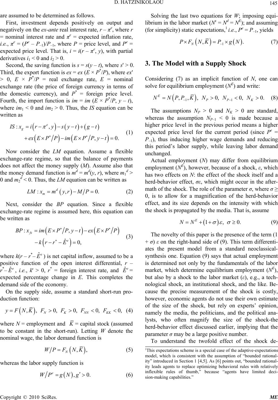

D. HATZINIKOLAOU
145
are assumed to be determined as follows.
First, investment depends positively on output and
negatively on the ex-ante real interest rate, r – πe, where r
= nominal interest rate and πe = expected inflation rate,
i.e., πe = (Pe – Ρ–1)/Ρ–1, where Ρ = price level, and Pe =
expected price level. That is, i = i(r – πe, y), with partial
derivatives i1 < 0 and i2 > 0.
Second, the saving function is s = s(y – t), where s' > 0.
Third, the export function is ex = ex (E × P*/P), where ex'
> 0, E × P*/P = real exchange rate, E = nominal
exchange rate (the price of foreign currency in terms of
the domestic currency), and P* = foreign price level.
Fourth, the import function is im = im (E × P*/P, y – t),
where im1 < 0 and im2 > 0. Thus, the IS equation can be
written as



:,
,0
e
g
ISxi rysytgt
exE PPimE PPy t


 
 .
(1)
Now consider the LM equation. Assume a flexible
exchange-rate regime, so that the balance of payments
does not affect the money supply (M). Assume also that
the money demand function is md = md(y, r), where m1
d >
0 and m2
d < 0. Thus, the LM equation can be written as

:,
d
m
LMxmy rMP0. (2)
Next, consider the BP equation. Since a flexible
exchange-rate regime is assumed here, this equation can
be written as


:,
ˆ0,
fx
e
BPximEPP ytexEPP
kr rE


 
 (3)
where k(r – r*–) is net capital inflow, assumed to be a
positive function of the open interest differential, r –
r*–, i.e., k' > 0, r* = foreign interest rate, and =
expected percentage change in E. This completes the
demand side of the economy.
ˆe
E
ˆe
Eˆe E
On the supply side, assume a standard short-run pro-
duction function:

, ,0,0,0,0,
NKNNKK
yFNK FFFF
(4)
where N = employment and
K
= capital stock (assumed
to be constant in the short-run). Letting W denote the
nominal wage, the labor demand function is


,
N
WPFNK, (5)
whereas the labor supply function is

,
e
WPgN g


Solving the last two equations for W; imposing equi-
librium in the labor market (Ns = Nd = NE); and assuming
(for simplicity) static expectations,1 i.e., Pe = P–1, yields



1
,.
N
PF NKPgN

 (7)
3. The Model with a Supply Shock
Considering (7) as an implicit function of N, one can
solve for equilibrium employment (NE) and write:


11
,,, 0,0,0.
E
PP K
NNPPKN NN

 (8)

The assumptions NΡ > 0 and NΚ > 0 are standard,
whereas the assumption NΡ–1 < 0 is made because a
higher price level in the previous period means a higher
expected price level for the current period (since Pe =
P–1), thus inducing higher wage demands and reducing
this period’s labor supply, while leaving labor demand
unchanged.
Actual employment (N) may differ from equilibrium
employment (NE), however, because of a shock, ε, which
has two effects on N: the effect of the shock itself and a
herd-behavior effect, σε, which might occur in the after-
math of the shock. The role of the parameter σ, where σ ≥
0, is to allow for a magnification of the herd-behavior
effect, and its size depends on the intensity with which
the shock is propagated by the media. That is, assume


1,
E
NN   0.

  (9)
The novelty of this paper is the presence of the term (1
+ σ) ε on the right-hand side of (9). This term differenti-
ates the present model from a standard neoclassical-
synthesis one. Equation (9) says that actual employment
is determined not only by the fundamentals of the labor
market, which determine equilibrium employment (NE),
but also by a shock to the labor market (ε), e.g., a tech-
nological shock, an institutional shock, and the like. Be-
cause the precise measurement of the shock is costly,
however, economic agents do not use their own estimate
of the size of the shock, but rely on experts’ opinion,
namely the media, the politicians, and the political ana-
lysts, who often magnify the size of the shock-the
herd-behavior effect discussed earlier, implying that the
parameter σ may be a large positive number.
To understand the twofold effect of the shock de-
1This expectations scheme is a special case of the adaptive-expectations
model, which is consistent with the assumption of “bounded rational-
ity” introduced in Section 1 [4,5]. As [6] points out, “bounded rational-
ity leads agents to replace optimizing behavioral rules with relatively
inflexible rules of thumb,” because “agents have limited deci-
sion-making capabilities.”
0. (6)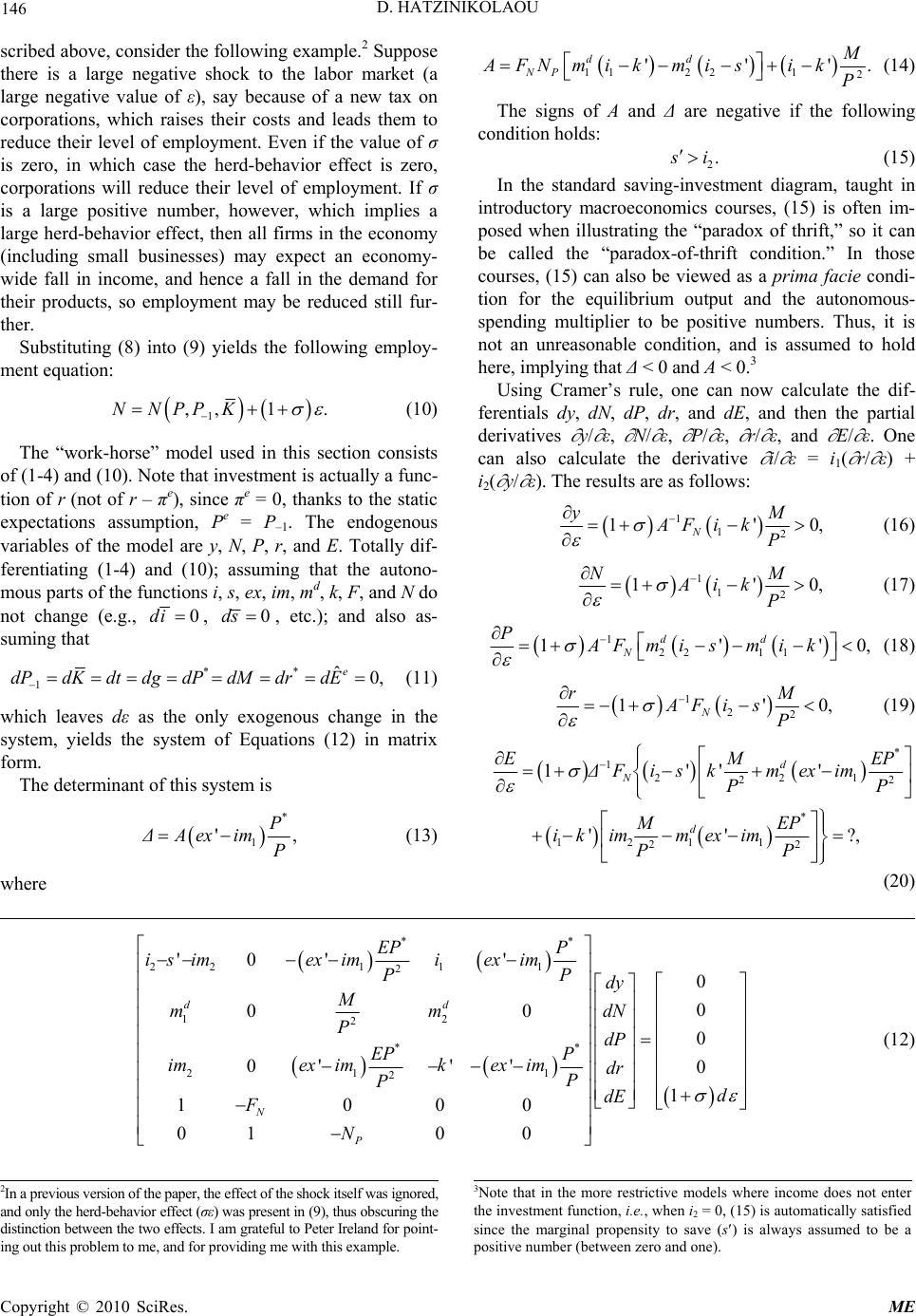

D. HATZINIKOLAOU
146
scribed above, consider the following example.2 Suppose
there is a large negative shock to the labor market (a
large negative value of ε), say because of a new tax on
corporations, which raises their costs and leads them to
reduce their level of employment. Even if the value of σ
is zero, in which case the herd-behavior effect is zero,
corporations will reduce their level of employment. If σ
is a large positive number, however, which implies a
large herd-behavior effect, then all firms in the economy
(including small businesses) may expect an economy-
wide fall in income, and hence a fall in the demand for
their products, so employment may be reduced still fur-
ther.

11221 2
'''.
M
dd
NP
AFNmi kmisi kP



(14)
The signs of A and Δ are negative if the following
condition holds:
2.
s
i

 (15)
In the standard saving-investment diagram, taught in
introductory macroeconomics courses, (15) is often im-
posed when illustrating the “paradox of thrift,” so it can
be called the “paradox-of-thrift condition.” In those
courses, (15) can also be viewed as a prima facie condi-
tion for the equilibrium output and the autonomous-
spending multiplier to be positive numbers. Thus, it is
not an unreasonable condition, and is assumed to hold
here, implying that Δ < 0 and A < 0.3
Substituting (8) into (9) yields the following employ-
ment equation:
Using Cramer’s rule, one can now calculate the dif-
ferentials dy, dN, dP, dr, and dΕ, and then the partial
derivatives  y/  ε,  N/  ε,  P/  ε,  r/  ε, and  Ε/  ε. One
can also calculate the derivative  i/  ε = i1(  r/  ε) +
i2(
 y/  ε). The results are as follows:


1
,, 1NNPPK .



 (10)
The “work-horse” model used in this section consists
of (1-4) and (10). Note that investment is actually a func-
tion of r (not of r – πe), since πe = 0, thanks to the static
expectations assumption, Pe = P–1. The endogenous
variables of the model are y, N, P, r, and E. Totally dif-
ferentiating (1-4) and (10); assuming that the autono-
mous parts of the functions i, s, ex, im, md, k, F, and N do
not change (e.g., 0di , 0ds , etc.); and also as-
suming that
 
1
12
1'
N
yM
AFik P



0,


 (16)
 
1
12
1'
NM
Aik
P



0,


 (17)

1
22 11
1'
dd
N
PAFm ism ik




'0,




(18)
**
1ˆ0,
e
dPdKdt dg dPdMdrdE
 (11)
 
1
22
1'
N
rM
AFis P



0,

 
 (19)
which leaves dε as the only exogenous change in the
system, yields the system of Equations (12) in matrix
form.
 
 
*
1
221
22
*
1211
22
1'''
''?
d
N
d
EM
ΔFisk mexim
PP
MEP
ik immexim
PP




 






 




,
EP
(20)
The determinant of this system is

*
1
'
P
ΔAex imP  , (13)
where
 
 

**
221 11
2
12
2
**
21 1
2
'0' '
0
0
00
0
0' ''0
1
1000
010 0
dd
N
P
EP P
isimex imiex imP
Pdy
MdN
mm
PdP
EP P
imex imkex imdr
P Pd
dE
F
N



 






























 








(12)
3Note that in the more restrictive models where income does not enter
the investment function, i.e., when i2 = 0, (15) is automatically satisfied
since the marginal propensity to save (s) is always assumed to be a
p
ositive number (between zero and one).
2In a previous version of the paper, the effect of the shock itself was ignored,
and only the herd-behavior effect (σε) was present in (9), thus obscuring the
distinction between the two effects. I am grateful to Peter Ireland for point-
ing out this problem to me, and for providing me with this example.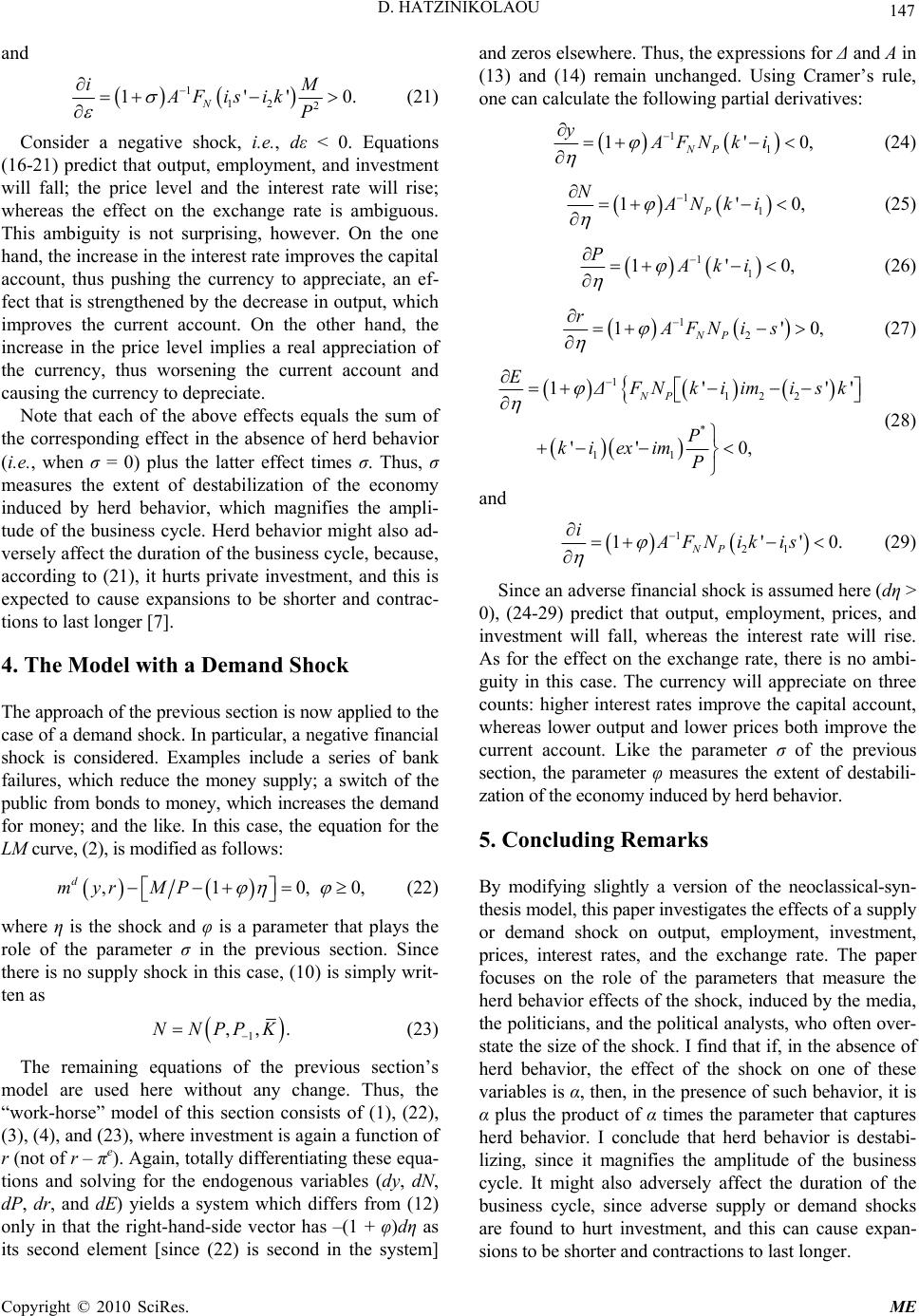

D. HATZINIKOLAOU
147
and
 
1
12 2
1''
N
i
AFisik P



 
0.
M
(21)
Consider a negative shock, i.e., dε < 0. Equations
(16-21) predict that output, employment, and investment
will fall; the price level and the interest rate will rise;
whereas the effect on the exchange rate is ambiguous.
This ambiguity is not surprising, however. On the one
hand, the increase in the interest rate improves the capital
account, thus pushing the currency to appreciate, an ef-
fect that is strengthened by the decrease in output, which
improves the current account. On the other hand, the
increase in the price level implies a real appreciation of
the currency, thus worsening the current account and
causing the currency to depreciate.
Note that each of the above effects equals the sum of
the corresponding effect in the absence of herd behavior
(i.e., when σ = 0) plus the latter effect times σ. Thus, σ
measures the extent of destabilization of the economy
induced by herd behavior, which magnifies the ampli-
tude of the business cycle. Herd behavior might also ad-
versely affect the duration of the business cycle, because,
according to (21), it hurts private investment, and this is
expected to cause expansions to be shorter and contrac-
tions to last longer [7].
4. The Model with a Demand Shock
The approach of the previous section is now applied to the
case of a demand shock. In particular, a negative financial
shock is considered. Examples include a series of bank
failures, which reduce the money supply; a switch of the
public from bonds to money, which increases the demand
for money; and the like. In this case, the equation for the
LM curve, (2), is modified as follows:
 
,10,
d
myr MP   

0,
(22)
where η is the shock and φ is a parameter that plays the
role of the parameter σ in the previous section. Since
there is no supply shock in this case, (10) is simply writ-
ten as

1
,,NNPPK



. (23)
The remaining equations of the previous section’s
model are used here without any change. Thus, the
“work-horse” model of this section consists of (1), (22),
(3), (4), and (23), where investment is again a function of
r (not of r – πe). Again, totally differentiating these equa-
tions and solving for the endogenous variables (dy, dN,
dP, dr, and dE) yields a system which differs from (12)
only in that the right-hand-side vector has –(1 + φ)dη as
its second element [since (22) is second in the system]
and zeros elsewhere. Thus, the expressions for Δ and A in
(13) and (14) remain unchanged. Using Cramer’s rule,
one can calculate the following partial derivatives:
 
1
1
1'
NP
yAFN ki



0,


 (24)
 
1
1
1'
P
NANk i



0,


 (25)
 
1
1
1'
PAki



0,


 (26)
 
1
2
1'
NP
rAFN is



0,


 (27)
 


 
1
122
*
11
1'
'' 0,
NP
EΔ''
F
Nkiim isk
P
kieximP




 






 


(28)
and
 
1
21
1'
NP
iAFN ikis



'0.


 (29)
Since an adverse financial shock is assumed here (dη >
0), (24-29) predict that output, employment, prices, and
investment will fall, whereas the interest rate will rise.
As for the effect on the exchange rate, there is no ambi-
guity in this case. The currency will appreciate on three
counts: higher interest rates improve the capital account,
whereas lower output and lower prices both improve the
current account. Like the parameter σ of the previous
section, the parameter φ measures the extent of destabili-
zation of the economy induced by herd behavior.
5. Concluding Remarks
By modifying slightly a version of the neoclassical-syn-
thesis model, this paper investigates the effects of a supply
or demand shock on output, employment, investment,
prices, interest rates, and the exchange rate. The paper
focuses on the role of the parameters that measure the
herd behavior effects of the shock, induced by the media,
the politicians, and the political analysts, who often over-
state the size of the shock. I find that if, in the absence of
herd behavior, the effect of the shock on one of these
variables is α, then, in the presence of such behavior, it is
α plus the product of α times the parameter that captures
herd behavior. I conclude that herd behavior is destabi-
lizing, since it magnifies the amplitude of the business
cycle. It might also adversely affect the duration of the
business cycle, since adverse supply or demand shocks
are found to hurt investment, and this can cause expan-
sions to be shorter and contractions to last longer.

148 D. HATZINIKOLAOU
Of course, in addition to herd behavior, other causes of
shock magnification might also be at work, thus turning
into a depression what would otherwise be only a mild
recession. Changes in attitudes, uncertainty about up-
coming government regulations, and other structural
changes that may be in operation simultaneously with the
shock, may influence its effect. For example,4 the three
most recent recoveries in the United States (1991, 2001,
and 2009-2010) have been dubbed “jobless recoveries”
because output growth was not accompanied by a sig-
nificant job growth, a phenomenon that can be explained
by an expansion in labor productivity. It is possible that
during these recessions and the ensuing recovery periods
managers altered their rehiring policies and that this ex-
tended the recovery periods and had nothing to do with
herd behavior. Reference [8] argues that job losses that
stem from structural changes (e.g., a permanent fall in
demand, technological change, reorganization of produc-
tion, and the like) are permanent, so the jobs added dur-
ing a recovery are mostly newly created positions, not
rehires. Creating new jobs, however, takes longer than
simply recalling laid-off workers, and is riskier because
at the beginning of a recovery there is a lot of uncertainty
whether the increase in demand will continue. Thus,
structural changes can prolong periods of high unem-
ployment, especially when there is no productivity growth.
6. Acknowledgements
I wish to thank an anonymous referee of this Journal for
his/her useful comments, which improved the paper. The
usual disclaimer applies.
7. References
[1] S. Mullainathan and A. Shleifer, “Media Bias,” NBER
Working Paper 9295, Cambridge, MA, 2002.
[2] K. J. Alsem, S. Brakman, L. Hoogduin and G. Kuper,
“The Impact of Newspapers on Consumer Confidence:
Does Spin Bias Exist?” Applied Economics, Vol. 40, No.
5, 2008, pp. 531-539.
[3] R. J. Shiller, “Conversation, Information, and Herd Be-
havior,” American Economic Review, Vol. 85, No. 2,
1995, pp. 181-185.
[4] J. Conlisk, “Why Bounded Rationality?” Journal of Eco-
nomic Literature, Vol. 34, No. 1, 1996, pp. 669-700 (a).
[5] G. W. Evans and G. Ramey, “Adaptive Expectations,
Underparameterization and the Lucas Critique,” Journal
of Monetary Economics, Vol. 53, No. 2, 2006, pp.
249-264.
[6] J. Conlisk, “Bounded Rationality and Market Fluctua-
tions,” Journal of Economic Behavior and Organization,
Vol. 29, No. 2, 1996, pp. 233-250 (b).
[7] V. Castro, “The Duration of Economic Expansions and
Recessions: More than Duration Dependence,” Journal of
Macroeconomics, Vol. 32, No. 1, 2010, pp. 347-365.
[8] E. L. Groshen and S. Potter, “Has Structural Change
Contributed to a Jobless Recovery? Federal Reserve Bank
of New York,” Current Issues in Economics and Finance,
Vol. 9, No. 8, 2003, pp. 1-7.
4In a previous version of the paper, there was no discussion of othe
r
p
ossible causes of shock magnification, in addition to herd behavior. I
am grateful to an anonymous referee of this Journal for suggesting that
I should include such a discussion and for providing me with this ex-
ample.