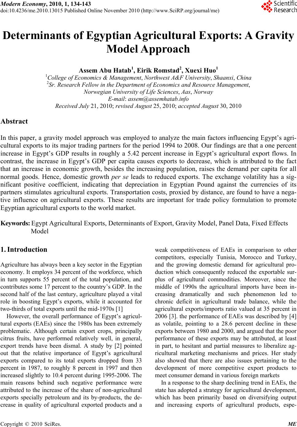
 Modern Economy, 2010, 1, 134-143 doi:10.4236/me.2010.13015 Published Online November 2010 (http://www.SciRP.org/journal/me) Copyright © 2010 SciRes. ME Determinants of Egyptian Agricultural Exports: A Gravity Model Approach Assem Abu Hatab1, Eirik Romstad2, Xuexi Huo1 1College of Economics & Management, Northwest A&F University, Shaanxi, China 2Sr. Research Fellow in the Department of Eco nomic s an d Resource Management, Norwegian University of Life Sciences, Aas, Norway E-mail: assem@assemhatab.info Received July 21, 201 0; revised August 25, 2010; accepted August 30, 2010 Abstract In this paper, a gravity model approach was employed to analyze the main factors influencing Egypt’ s agri- cultural exports to its major trading partners for the period 1994 to 2008. Our findings are that a one percent increase in Egypt’s GDP results in roughly a 5.42 percent increase in Egypt’s agricultural export flows. In contrast, the increase in Egypt’s GDP per capita causes exports to decrease, which is attributed to the fact that an increase in economic growth, besides the increasing population, raises the demand per capita for all normal goods. Hence, domestic growth per se leads to reduced exports. The exchange volatility has a sig- nificant positive coefficient, indicating that depreciation in Egyptian Pound against the currencies of its partners stimulates agricultural exports. Transportation costs, proxied by distance, are found to have a nega- tive influence on agricultural exports. These results are important for trade policy formulation to promote Egyptian agricultural exports to the world market. Keywords: Egypt Agricultural Exports, Determinants of Export, Gravity Model, Panel Data, Fixed Effects Model 1. Introduction Agriculture has always been a key sector in the Egyptian economy. It employs 34 percent of the workforce, which in turn supports 55 percent of the total population, and contributes some 17 percent to the country’s GDP. In the second half of the last century, agriculture played a vital role in boosting Egypt’s exports, while it accounted for two-thirds of total exports until the mid -1970s [1] However, the overall performance of Egypt’s agricul- tural exports (EAEs) since the 1980s has been extremely problematic. Although certain export crops, principally citrus fruits, have performed relatively well, in general, export trends have been dismal. A study by [2] pointed out that the relative importance of Egypt’s agricultural exports compared to its total exports dropped from 33 percent in 1987, to roughly 8 percent in 1997 and then increased slightly to 10.4 percent during 1995-2006. The main reasons behind such negative performance were attributed to the increase of the share of non-agricultural exports specially petroleum and its by-products, the de- crease in quality of agricultural exported products and a weak competitiveness of EAEs in comparison to other competitors, especially Tunisia, Morocco and Turkey, and the growing domestic demand for agricultural pro- duction which consequently reduced the exportable sur- plus of agricultural commodities. Moreover, since the middle of 1990s the agricultural imports have been in- creasing dramatically and such phenomenon led to chronic deficit in agricultural trade balance, while the agricultural exports/imports ratio valued at 35 percent in 2006 [3]. the performance of EAEs was described by [4] as volatile, pointing to a 28.6 percent decline in these exports between 1980 and 2000, and argu ed that the poor performance of these exports may be attributed, at least in part, to hesitant and partial measures to liberalize ag- ricultural marketing mechanisms and prices. Her study also showed that there are also issues pertaining to the development of more competitive export products to meet consumer demand in various foreign markets In a response to the sharp declining trend in EAEs, the state has adopted a strategy for agricultural development, which has been primarily based on diversifying output and increasing exports of agricultural products, espe- 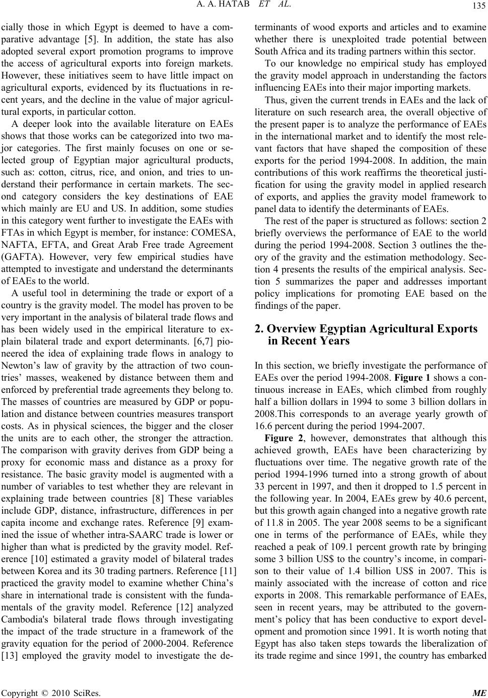 A. A. HATAB ET AL. 135 cially those in which Egypt is deemed to have a com- parative advantage [5]. In addition, the state has also adopted several export promotion programs to improve the access of agricultural exports into foreign markets. However, these initiatives seem to have little impact on agricultural exports, evidenced by its fluctuations in re- cent years, and the decline in the value of major agricul- tural exports, in particular cotton. A deeper look into the available literature on EAEs shows that those works can be categorized into two ma- jor categories. The first mainly focuses on one or se- lected group of Egyptian major agricultural products, such as: cotton, citrus, rice, and onion, and tries to un- derstand their performance in certain markets. The sec- ond category considers the key destinations of EAE which mainly are EU and US. In addition, some studies in this category went further to investigate the EAEs with FTAs in which Egypt is member, for instance: COMESA, NAFTA, EFTA, and Great Arab Free trade Agreement (GAFTA). However, very few empirical studies have attempted to investigate and understand th e determinants of EAEs to the world. A useful tool in determining the trade or export of a country is the gravity model. The model has proven to be very important in the analysis o f bilateral trade flows and has been widely used in the empirical literature to ex- plain bilateral trade and export determinants. [6,7] pio- neered the idea of explaining trade flows in analogy to Newton’s law of gravity by the attraction of two coun- tries’ masses, weakened by distance between them and enforced by preferential trade agreements they belong to. The masses of countries are measured by GDP or popu- lation and distance between countries measures transport costs. As in physical sciences, the bigger and the closer the units are to each other, the stronger the attraction. The comparison with gravity derives from GDP being a proxy for economic mass and distance as a proxy for resistance. The basic gravity model is augmented with a number of variables to test whether they are relevant in explaining trade between countries [8] These variables include GDP, distance, infrastructure, differences in per capita income and exchange rates. Reference [9] exam- ined the issue of whether intra-SAARC trade is lower or higher than what is predicted by the gravity model. Ref- erence [10] estimated a gravity model of bilateral trades between Korea and its 30 trading partners. Reference [11] practiced the gravity model to examine whether China’s share in international trade is consistent with the funda- mentals of the gravity model. Reference [12] analyzed Cambodia's bilateral trade flows through investigating the impact of the trade structure in a framework of the gravity equation for the period of 2000-2004. Reference [13] employed the gravity model to investigate the de- terminants of wood exports and articles and to examine whether there is unexploited trade potential between South Africa and its trading partners within this sector. To our knowledge no empirical study has employed the gravity model approach in understanding the factors influencing EAEs into their major importing markets. Thus, given the current trends in EAEs and the lack of literature on such research area, the overall objective of the present paper is to analyze the performance of EAEs in the international market and to identify the most rele- vant factors that have shaped the composition of these exports for the period 1994-2008. In addition, the main contributions of this work reaffirms the theoretical justi- fication for using the gravity model in applied research of exports, and applies the gravity model framework to panel data to identify the determinants of EAEs. The rest of the paper is structured as follows: section 2 briefly overviews the performance of EAE to the world during the period 1994-2008. Section 3 outlines the the- ory of the gravity and the estimation methodology. Sec- tion 4 presents the results of the empirical analysis. Sec- tion 5 summarizes the paper and addresses important policy implications for promoting EAE based on the findings of the pape r. 2. Overview Egyptian Agricultural Exports in Recent Years In this section, we briefly investigate the p erformance of EAEs over the p eriod 1994-2008 . Figure 1 shows a con- tinuous increase in EAEs, which climbed from roughly half a billion dollars in 1994 to some 3 billion dollars in 2008.This corresponds to an average yearly growth of 16.6 percent during the period 1994-2007. Figure 2, however, demonstrates that although this achieved growth, EAEs have been characterizing by fluctuations over time. The negative growth rate of the period 1994-1996 turned into a strong growth of about 33 percent in 1997, and then it dropped to 1.5 percent in the following year. In 2004, EAEs grew by 40.6 percent, but this growth again changed into a negative growth rate of 11.8 in 2005. The year 2008 seems to be a significant one in terms of the performance of EAEs, while they reached a peak of 109.1 percent growth rate by bringing some 3 billion US$ to the country’s in come, in compari- son to their value of 1.4 billion US$ in 2007. This is mainly associated with the increase of cotton and rice exports in 2008. This remarkable performance of EAEs, seen in recent years, may be attributed to the govern- ment’s policy that has been conductive to export devel- opment and promotion since 1991. It is worth noting that Egypt has also taken steps towards the liberalization of its trade regime and since 1991, the country has embarked Copyright © 2010 SciRes. ME 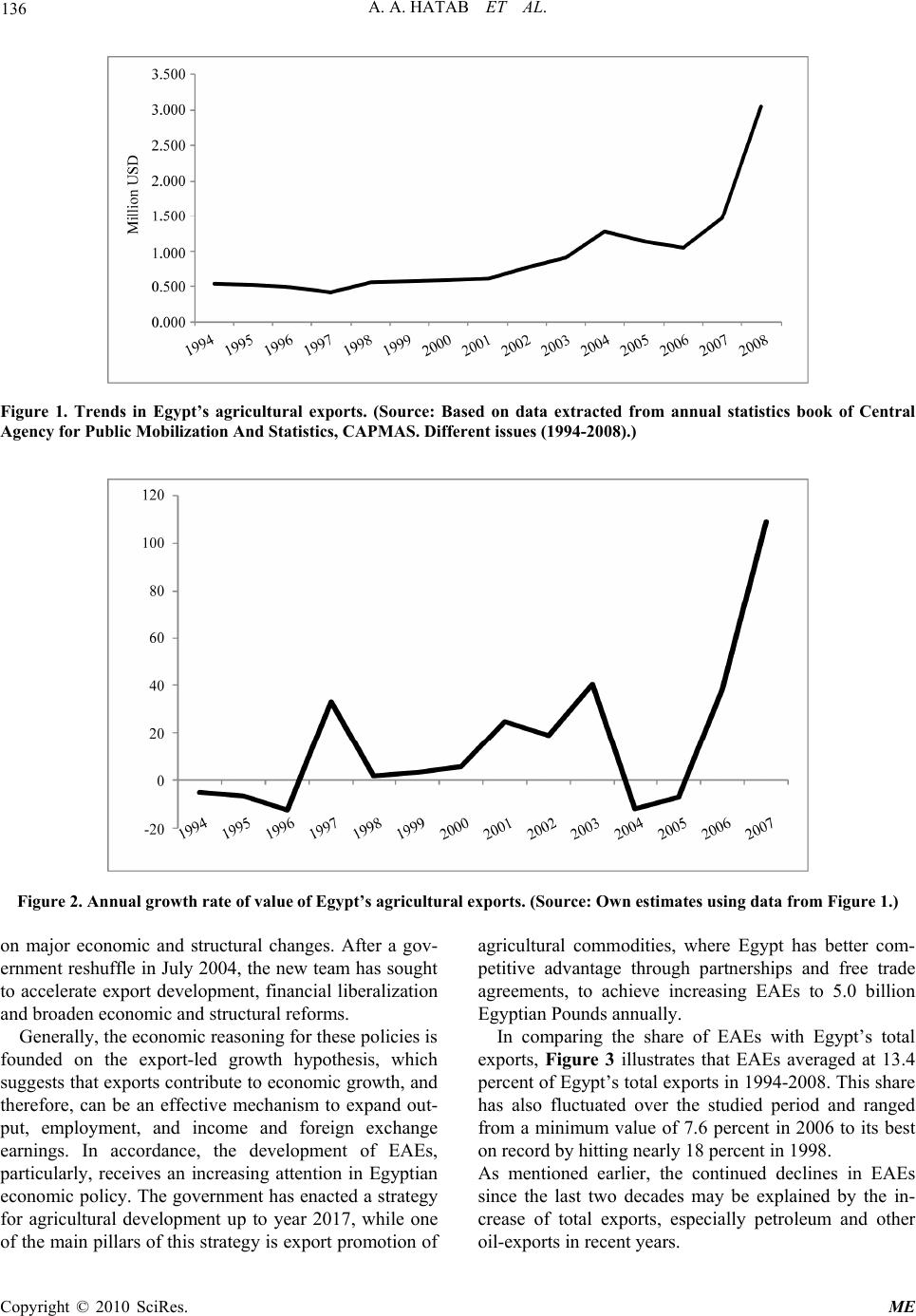 A. A. HATAB ET AL. Copyright © 2010 SciRes. ME 136 Figure 1. Trends in Egypt’s agricultural exports. (Source: Based on data extracted from annual statistics book of Central Agency for Public Mobilization And Statistics, CAPMAS. Different i s sues (1994-2008).) Figure 2. Annual growth rate of value of Egypt’s agricultural exports. (Source: Own estimates using data from Figure 1.) on major economic and structural changes. After a gov- ernment reshuffle in July 2004, the new team has sought to accelerate export development, financial liberalization and broaden economic and structural reforms. Generally, the economic reasoning for these policies is founded on the export-led growth hypothesis, which suggests that exports con tribute to economic growth, and therefore, can be an effective mechanism to expand out- put, employment, and income and foreign exchange earnings. In accordance, the development of EAEs, particularly, receives an increasing attention in Egyptian economic policy. The government has enacted a strategy for agricultural development up to year 2017, while one of the main pillars of this strategy is export promotion of agricultural commodities, where Egypt has better com- petitive advantage through partnerships and free trade agreements, to achieve increasing EAEs to 5.0 billion Egyptian Pounds ann ually. In comparing the share of EAEs with Egypt’s total exports, Figure 3 illustrates that EAEs averaged at 13.4 percent of Eg ypt’s total exports in 1994- 2008. This shar e has also fluctuated over the studied period and ranged from a minimum value of 7.6 percent in 2006 to its best on record by hitting n early 18 percent in 1998. As mentioned earlier, the continued declines in EAEs since the last two decades may be explained by the in- crease of total exports, especially petroleum and other oil-exports in recent years. 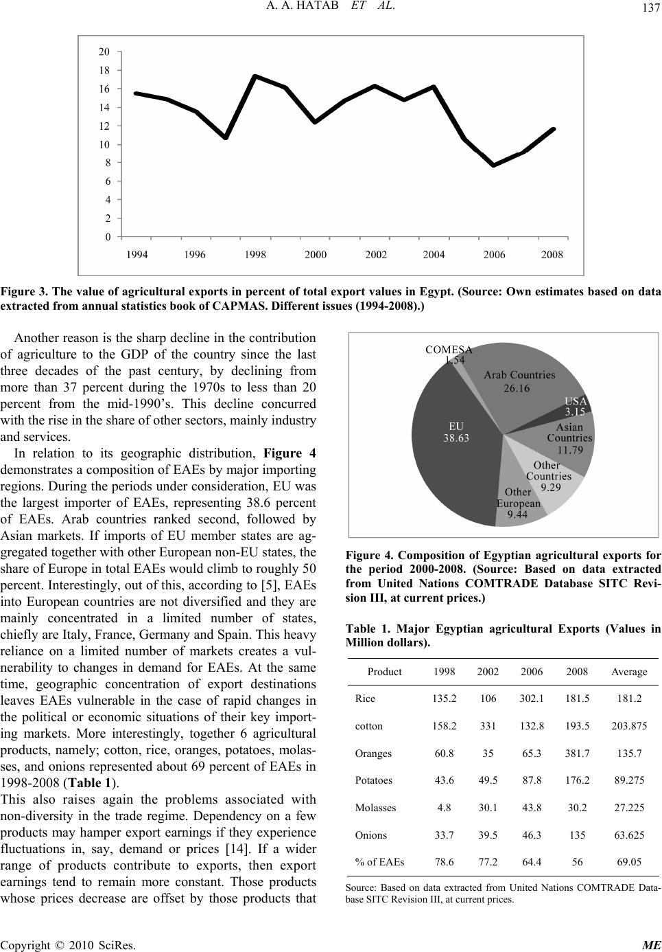 A. A. HATAB ET AL. 137 Figure 3. The value of agricultural exports in percent of total export values in Egypt. (Source: Own estimates based on data extracted from annual statistics book of CAPMAS. Different issues (1994-2008).) Another reason is the sh arp decline in the contribution of agriculture to the GDP of the country since the last three decades of the past century, by declining from more than 37 percent during the 1970s to less than 20 percent from the mid-1990’s. This decline concurred with the rise in the share of other sectors, mainly industry and services. In relation to its geographic distribution, Figure 4 demonstrates a composition of EAEs by major importing regions. During the periods under consideration, EU was the largest importer of EAEs, representing 38.6 percent of EAEs. Arab countries ranked second, followed by Asian markets. If imports of EU member states are ag- gregated together with other European non-EU states, the share of Europe in total EAEs would climb to roughly 50 percent. Interestingly, out of this, according to [5], EAEs into European countries are not diversified and they are mainly concentrated in a limited number of states, chiefly are Italy, France, Germany and Spain. This heavy reliance on a limited number of markets creates a vul- nerability to changes in demand for EAEs. At the same time, geographic concentration of export destinations leaves EAEs vulnerable in the case of rapid changes in the political or economic situations of their key import- ing markets. More interestingly, together 6 agricultural products, namely; cotton, rice, oranges, potatoes, molas- ses, and onions represented about 69 percent of EAEs in 1998-2 00 8 (Table 1). This also raises again the problems associated with non-diversity in the trade regime. Dependency on a few products may hamper export earnings if they experience fluctuations in, say, demand or prices [14]. If a wider range of products contribute to exports, then export earnings tend to remain more constant. Those products whose prices decrease are offset by those products that Figure 4. Composition of Egyptian agricultural exports for the period 2000-2008. (Source: Based on data extracted from United Nations COMTRADE Database SITC Revi- sion III, at current prices.) Table 1. Major Egyptian agricultural Exports (Values in Million dollars). Product 1998 20022006 2008 Average Rice 135.2106 302.1 181.5 181.2 cotton 158.2331 132.8 193.5 203.875 Oranges 60.8 35 65.3 381.7 135.7 Potatoes 43.6 49.5 87.8 176.2 89.275 Molasses 4.8 30.1 43.8 30.2 27.225 Onions 33.7 39.5 46.3 135 63.625 % of EAEs 78.6 77.2 64.4 56 69.05 Source: Based on data extracted from United Nations COMTRADE Data- base SITC Revision III, at current price s. Copyright © 2010 SciRes. ME  138 A. A. HATAB ET AL. experience prices increases. Furthermore, if there are only a small number of export-oriented industries, and they become unstable, then investment in them may be withdrawn and this negativ ely affects growth [15]. It is also noticeable that these products are exported as row material or fresh products with almost no processing operations. According to [16], vertical diversification of exports which occurs when the composition of exports shift from primary products to manufactured products. Vertical export diversification contributes to stabilization in export earnings, as the prices of manufactured exports do not fluctuate as much as those of primary exports. 3. Factors Influencing Egypt’s Agricultural Exports 3.1. Foundation of the Model To provide a comprehensive empirical analysis of EAEs flow to the world wide, the well known gravity model has been employed. This model developed simultane- ously by Tinbergen (1962) [6] as well as Pöyhönen (1963) [7] and Pulliainen (1963) [17] is actually consid- ered as one of the most fruitful ways to formalize and explain bilateral trade flows [18,19]. According to the Law of universal gravitation discovered by Newton in 1687, the standard gravity model simply describes that the trade between two countries is determined positively by each country’s GDP, and negatively by the distance between them. This formulation can be generalized as follows: 12 3 0iji jij YY D (1) where ij is the flow of exports into country j from country i , and i Y Y are country i’s and country j’s GDPs and ij is the geographical distance between the countries’ capitals. D The linear form of the model is as follows: 12 3 loglog loglog ijij ij YY Y (2) he generalized gravity model of trade states that the vo- lume of exports between pairs of countries, ij , is a function of their incomes (GDPs), their populations, their distance (proxy of transportation costs) and a set of dummy variables either facilitating or restricting trade between pairs of countries. That is, 123456 0ij ijijij ij ij YY LLDAeu (3) where i (Y Y) indicates the GDP of the country i (j), i (L L) are populations of the country i (j), ij meas- ures the distance between the two countries’ capitals (or economic centers), ij D represents dummy variables, is the error term and ij eu s are parameters of the model. 3.2. Specification of the Model The model we develop is focused specifically on Egyp- tian agricultural products. For this reason it is necessary to take into account the geographical structure of Egyp- tian agricultural exports as described above. Following the extensive literature produced at least during the last 20 years relatively to the gravity model, the equation used in the present work is an augmented form of the basic gravity equation. Reference [20] pointed out that additional variables might be added to impro ve the basic formulation of the selected gravity equation, while this addition of variables gives us the possibility of adopting the gravity equation to the particular circumstances of the bilateral trade under study. Thus, we have added some additional variables as explanatory variables in order to better understanding of EAE flows. More pre- cisely, the volume of EAEs depends on the discussed below varia bl es. Income is one of the most traditio nal enhancement va- riables in bilateral trade. Reference [21] argued that the GDP must be the proper measure of the country’s poten - tial trade. The GDP of the exporting country (Egypt) measures productive capacity, while that of the import- ing country measures absorptive capacity. These two variables are expected to be positively related to trade [22]. We also included variables of GDP per capita of importers and Egypt. It is expected that the higher the income per capita for a cou ntry j, the greater the demand for imports, and thus Egypt’s agricultural exports. This model has included distance as a proxy of trans- action costs–including transportation costs. The most popular absolute geographical distance variable is the distance between capitals, as a proxy for the economic center of a country. An increase in distance between countries is expected to increase transportation costs, thus reducing trade. This variable is expected to be nega- tive [23]. Openness is an element that makes a difference in the formulation of traditional gravity equations. Openness is the indicator of total exports plus total imports over GDP, Openness = (total exports + total imports)/real GDP. EAEs to their major trading partners could increase or decrease with the level of openness [24] Reference [21] added the real bilateral exchange rate in their empirical model as an explanatory variable in examining Mercosur-EU trade flows. The actual bilateral exchange rate is defined in this paper as the number of the importing market units of currency that can be pur- chased by one Egyptian pound. The coefficient of the actual bilateral exchange rate is expected to be negative. Copyright © 2010 SciRes. ME  A. A. HATAB ET AL. 139 This paper introduces dummy variables (included in ij ) to represent various regional trade agreements (RTA), common language and common borders. The dummy variables take the value one if the importing market has a signed free trade agreement with Egypt, if Arabic is the official language of country j, and if Egypt and country j share a common border. Otherwise, they take the value of zero. Therefore, the value of agricultural exports (ij ) from Egypt i to its major trading partners js is defines as fol- lows: 1234567 8 0 91011 ijij i jijijij ij ij ijij YYLL OPOPExrD RTA CommonBCommonLeu (4) Where 0 A is a constant, Y is the GDP, L is the pop - ulation, Op is the real openness, Exr is the real bilateral exchange rate, D is the distance, and RTA, Common B, and Common L are dummy variables of regional trade agreement, common border, and common language, re- spectively. We transform equation 4 to a linear form 5 by logarithmic transformation. For estimation panel data, this model would be re written as the following log-linear equation: 01 23 45 6 789 10 11 ... .. . ... .. ijij i ji j ij ijij ijij ij LnXLn YLn YLnL LnLLnOP LnOP Ln ExrLn DLn RTA Ln CommonBLn CommonLeu (15) 3.3. Estimation Methodology Panel data involves different models that can be esti- mated. These are pooled, fixed effects and random ef- fects. The main problem of the pooled model is that it does not allow for heterogeneity of countries. It does not estimate country specific effects and assumes that all countries are homogenous [25]. It is a restricted model. A random effects model can be more appropriate when estimating the flows of trade between a randomly sample drawn of trading partners from a large population. A fixed effects model would be a better model when esti- mating the flows of trade between ex ante predetermined selection of countries [8,26]. Since this study deals with the agricultural export flows of Egypt to its 50 main im- porting markets, the fixed effects model will be a more appropriate model than the random effect specification. Furthermore, we also apply the Hausman test to check whether the fixed effects model is more efficient than the random effects model. This will be true if the null hy- pothesis of no correlation between the individual effects and the regressors is rejected [15,27]. The fixed effects model has a problem in the sense that variables that do not change over time cannot be estimated directly because inherent transformation wipes out such variables. To solve this problem, these variables can be estimated in a second step by estimating another regression with the individual effects as the dependent variable and distance and dummy variables as independ- ent variables. This is specified as follows: 01 23 4 ijij ijij ij ij EDRTACommon CommonL eu B (6) where ij is individual effects, and other variables are as defined before. E 3.4. Data In our estimation, we study the EAEs into 50 importing markets during the period 1994-2008. The selection of these countries is based on the distribution of EAEs by country of destination during the period 2004-2008. Pri- mary analysis showed that 96 countr ies impor ted roug hly 95.6 percent of EAE during this period. The top 50 countries, out o f these 96 ones, imported 94.4 percent of EAE. Based on this, our estimation will be focusing on these top 50 importing countries. The selection of the period 2004 to 2008 is attributed to that fact that this period witnessed a substantial reform program in the Egyptian foreign trade sector and agricultural sector, along with the availability of data In sum, the annual data covers 50 countries for the years 1994 to 2008 with one dependant variable and 11 explanatory variables (a total of n = 750, N = 50, and T = 15), and all variables are expressed in natural logarithm. The data of GDP were collected from UNCTAD handbook of statistics. Data on population size were col- lected from the FAO website. The calculation of the de- gree of openness was based on the data from UNCTAD and the WAITS (World Bank Integrated Trade Solution) database [28]. Exchange rate data were gathered from the IMF website. The webpage of Travel Distance Calcula- tor between Cities was used in calculating the distance between Cairo and the capital cities of the studied coun- tries. Egyptian economic and statistical data, and infor- mation about its trade agreements were obtained from; Central Agency for Public Mobilization and Statistics (CAPMAS) [29], the off icial website of Egyp tian Minis- try of Trade and Industry. 3.5. Univariate Characteristics of Variables Before the estimation of Equation (5) the paper analyzed the univariate characteristics of the variables which entail Copyright © 2010 SciRes. ME  140 A. A. HATAB ET AL. panel unit root tests. This is the first step in determining a potentially cointegrated relationship between the vari- ables. If all variables are stationary, then the traditional estimation can be used to estimate the relationship be- tween variables. If they contain a unit root or are nonsta- tionary, a cointegration test should be performed [30]. This study applies two panel unit root tests using the LLC method [31], and IPS method [32]. The LLC test assumes that the autoregressive parameters are common across cross sections. It uses the null hypothesis of a unit root. The second test (IPS), however, allows the autore- gressive to vary across countries and also for individual unit root processes. It is computed by combining indi- vidual countries’ unit root tests to come up with a result that is specific to a panel. The null hypothesis is that all series contain a unit root test and the alternative is that at least one series in the panel contains a unit root. The results presented in Table 2 imply that both the LLC and IPS reject the null of unit root fo r all variables. That means all variables are stationary and this implies that co-integration test is not required and Equation (2) can be estimated using the ordinary least square method. 4. Empirical Results The estimation results of the gravity equation are pre- sented in Table 3. The pooled panel data results are in the second column of Table 3. As we stated before, the pooled model problems because it does not allow for heterogeneity of countries and country specific effects are not estimated. Results of the fixed effects model are presented in column 3. The fixed effects model intro- duces heterogeneity by estimating country specific ef- fects. It is an unrestricted model as it allows the intercept and other parameters to vary across trading partners. The F-test statistic was performed to test the ability to pool data and the results in Table 3 indicate that the null hy- pothesis of equality of ind ividual effects is rejected. This means that a model with individual effects is better than the pooled model. Like the fixed effects model, the random effects model also acknowledges heterogeneity in the cross-section. However, it differs from the fixed effects model in the sense that the effects are generated by a specific distribu- tion. Although it assumes that there is heterogeneity in the cross-section, it does not model each effect explicitly. This prevents the loss of degrees of freedom which takes place in fixed effects model. The LM test was per- formed and the null hypothesis of equality of the indi- vidual effects is rejected in favor of random effects specification (Table 3). The Hausman statistic is used to test the null hypothe- sis that the regressors and individual effects are not cor- Table 2. Panel unit root test. Test LLC IPS Agricultural exports -15.1061(0.000) *** - 4.062(0.000) *** Importer’s GDP -17.6065(0.000) *** - 1.545(0.061) * Egypt’s GDP -2.542(0.006) *** -1.524(0.062) * Importer’s G DP per capita-25.151(0.000) *** -2.620(0.004) *** Egypt’s GDP per capita -8.362(0.000) *** -3.759(0.000) *** Openness -8.8550(0.000) *** -4.3579(0.000) *** Exchange rate -7.9541(0.00 0 ) *** -4.065(0.000) *** Notes: ***/**/* denotes rejection of the at 1%/5%/10% level. Probabilities are in parenthesis. related in order to distinguish between fixed effects model and random effects model. Failure to reject the null hypothesis implies that the random effects model will be preferred. If the null hypothesis is rejected, the fixed effects model will be appropriate. The results in Table 3 show that the Hausman specificatio n test rejects the null hypothesis and this indicates that country spe- cific effects are correlated with regressors. This suggests that the fixed effects model is preferred. Since the fixed effects model is the appropriate one, interpretation of th e results will focus on the fixed effects model. The results of the fixed effects model as shown in Ta- ble 3 indicate that an increase in Egypt’s GDP causes an increase in EAEs. The highly significant coefficient of Egypt’s GDP is positive with estimated value of 5.42. This means that, holding constant for o ther variables; a 1 percent point increase in Egypt’s GDP will result in, roughly, a 5.42 percent point increase in EAEs flows. This result is consisten t with the basic assumption of the gravity model that states the trade volumes will increase with an increase in economic size. Although, the positive sign of the coefficient of the importer’s GDP, it is not statistically significant. This means that it cannot be considered as an explanatory variable for the demand for EAEs. In all the three estimated models, the coefficient of im- porter’s GDP per capita is negative. This indicates that an increase in the GDP per capita of the importing coun- try causes EAEs to decrease, but the coefficient is not statistically significant. This suggests that importer’s GDP per capita has no significant impact on exports. It also emphasizes that EAEs patterns follow a GDP pat- tern, concentrating on the production and export of quan- tity-based products and depending on overall market size, rather than a per capita GDP pattern centering on the export of quality-based high value added products wh ich are sensitive to the levels of income. Copyright © 2010 SciRes. ME  A. A. HATAB ET AL. Copyright © 2010 SciRes. ME 141 Table 3. Gravity model estimation results. Variable Pooled Regression Fixed Effects Model Random Effects model Constant -15.1008 (-1.85) * -22.0803 (-3.22)** -15.87991 (-1.94)* Importer’s G DP 0.7401 (7.40)*** 2.3386 (1.58) 0.7534 (7.66)*** Egypt’s GDP 5.7285 (3.59) ** 5.4238 (3.04)** 5.8771 (3.85)*** Importer GDP Per Capita -0.8132 (-0.64) -1.7663 (-1.23) -0.0445 (-0.24) Egypt’s GDP per capita -5.7817 (-3.48)** -5.9300 (-3.11)** -6.07 (-3.75)*** Importer Openness 0.1909 (-0.0 8) -0.1299 (-0.30) -0.0715 (-0.19) Egypt’s Openness 0.3340 (1.11) 0.6924 (1.46) 0.3905 (1.23) Exchange rate -0.0399 (-0.5 2) 0.4592 (3.58)** 0.1116 (1.08) Distance -1.1128 (-3.96)*** - -1.0726 (-3.73)*** Common Border 0.8636 (2.46)* - 1.0106 (2.63)** Common Language 0.9593 (2.81)** - 0.9523 (2.69)** RTA 0.0705 (0.18) - 0.5051 (0.95) NO. of Observation 750 750 750 Adjusted R2 0.55 0.59 0.51 F-test - 42.33*** - LM - - 289.834*** Hausman test - 30.64*** - Notes: ***/**/* significant at 1 %, 5%, and 10% level. All other var iables are statistically insigni ficant. t-statistics are in parenthesis. An increase in Egypt’s GDP per capita also causes exports to decrease. The coefficient of this variable shows strong negative and significant sign and this is not in line with the theory. The negative coefficient can be attributed to the accelerated economic growth rate in Egypt which reached 7 percent in the last decade, ac- companied with the increasing population of the coun try. Together these two factors can expand consumption, so the domestic market will absorb a greater part of the production, and this therefore reduces the surplus avail- able for export. Egypt’s openness and importers open- ness do not show significant coefficients, and thus are not explanatory variables in the EAEs to the world. The exchange volatility has a significant positive coefficient, indicating that depreciation in Egyptian Pound against the currencies of its partners stimulates agricultural ex- ports. The second stage regression results as explained in Equation (6) are presented in Table 4. Distance has the expected sign and is highly significant. Transportation cost is relevant to distances and trade falls with increas- ing physical distance between the countries. Hence one of the policy suggestions is that Egypt should make ef- forts to reduce transaction costs of trade with neighbor countries and economic blocs, such as Arab countries, COMESA and EU, so as to achieve a deeper economic integration. Countries where Arabic is the official language are associated with an increase Egyptian exports of agricul- tural products. It appears that the regional economic grouping which is expressed by the RTA dummy variab le is insignificant but positive and the fact that a country is a member of Table 4. Second stage regression: fixed effects regressed on dummies. Explanatory Variables Coefficient Distance -2.3699(-3.36)** Common Border -0.3504(-0.24) Common Language 2.4721(2.03)* RTA 1.6148(1.53) Adjusted R- square d 0.4376 Notes: **/* significant at 5%, and 10% level. t-stat istics are in parenthesis.  142 A. A. HATAB ET AL. RTA with Egypt does not seem to determine the ex- port volume. This implies that trade gains from the re- gional trade agreements have been minimal. Countries where Arabic is the official language are associated with an increase Egyptian exports of agricul- tural products. It appears that the regional economic grouping which is expressed by the RTA dummy vari- able is insignificant bu t positive and the fact that a coun- try is a member of RTA with Egypt does not seem to determine the export volume. This implies that trade gains from the regional trade agreements have been minimal. 5. Summary and Concluding Remarks Recognizing the impor tance of agricultural exports in the Egyptian economy, our study attempted to analyze EAE patterns empirically and to identify the factors influenc- ing EAEs into their major importing markets. More specifically, we employed the gravity model, which is considered one of the most efficient models in explaining bilateral trade, to EAEs covering the period 1994 to 2008 in order to investigate the factors that de- termine export flows of agricultural products from Egypt to its 50 major trading partners. Regression analysis was performed in three ways, which include the common intercept model, the fixed effects model, and the random effects model. When choosing between fixed and random effects, the Haus- man test rejected the null hypothesis (random effects were efficient). Therefore, the paper demonstrated that the fixed effects model generated the most reliable re- sults and then interpreted the results using this model. According to our results in this study, EAEs patterns follow the basic gravity model, implying that bilateral trade flows will increase in proportion to the trading partner’s GDP and decrease in proportion to the distance involved. Therefore, in order to expand bilateral trade flows, it appears to be more desirable for Egypt to pro- mote exports to countries in close proximity and having large economies. Importers’ Per capita GDP, in contrast, turned out to be an insignificant factor in determining EAEs. This implies that Egypt’s trade patterns follow a GDP pattern, concentrating on the production and export of quantity-based products and depending on overall market size, rather than a per capita GDP pattern center- ing on the export of quality-based high value added products which are sen sitive to the levels of income. The exchange rates in this paper were defined as the value of the partner country’s currency in terms of those of the Egyptian currency. The results suggest indicate that de- preciation in Egyptian Pound against the currencies of its partners stimulates agricultural exports. The variable of distance indicates that if distance be- tween Egypt and its major importing markets were re- duced, the expected change in agricultural export value would be positive. Thus, logistics are important in the export process, which could be increased by improved connections such as infrastructure, direct air travel and improved maritime transportation between Egypt and its trading part ner s . Results also imply that Egypt’s agricultural exports tend to increase into countries where the official lan- guage is Arabic, which suggests that sharing the same language promotes exports. This raises the importance for Egypt to expand and promote its agricultural exports to those countries. Membership of regional trade agreements does not encourage EAEs. The insignificance of regional eco- nomic groupings may be constrained by problem of sim- ilar comparative advantages, consumption issues, over- lapping membership, policy harmonization and poor private sector participation. Lastly, the results of the application of the gravity model to EAEs are quite supportive for th e configuration of policy recommendations which can improve the per- formance of EAEs in the international markets. These policy recommendations although crucial for the devel- opment of this sector, cannot be based upon the findings of the gravity model alone. Quite important role in this development procedure plays the internal environment with its positive and negative aspects, forming the quan- tity and quality characteristics of Egypt’s agricultural exports. Therefore, we recommend more detailed re- search on the internal environment and its influence on agricultural export performance. It is also possible that if more disaggregated data were used, a different result might emerge. We leave these topics for future research. 6. References [1] S. Mohammed, “The Future of Egyptian Agriculture in International Trade,” Working Paper Options Méditer- ranéennes, No. 9, 1995, Paris. [2] G. Shehata, “An Economic Study for Egyptian Foreign Agricultural Trade with Emphases on Relationship with European Union,” The second conference on economical competitiveness, quality of life, and sustainability, ka- posvár, 2009, pp. 68-79. [3] A. Hamdi, G. Mohamed and Z. Ezzat, “Analysis of Egyptian Grapes Market Shares in the World Markets,” American-Eurasian Journal of Agriculture and Environ- mental Science, Vol. 3, No. 4, 2008, pp. 656-662. [4] M. Sarah, “A Socio-Economic Profile of Egypt: Agricul- ture (1980-2002),” Working Paper Centre for Project Evaluation & Macroeconomic Analysis, No. 18, Cairo, 2003. Copyright © 2010 SciRes. ME  A. A. HATAB ET AL. Copyright © 2010 SciRes. ME 143 [5] A. Assem, G. Ahmed, H. Ragab and A. Soad, “Economic Study on Egyptian Agricultural Exports with Reference to North-Sinai Province’S Exports,” Master Dissertation, Suez Canal University, Al-Arish, February 2007. [6] J. Tinbergen, “Shaping the World Economy. Suggestion for an International Economic Policy,” Twentieth Cen- tury Fund, New York, 1962. [7] P. Pöyhönen, “A Tentative Model for the Volume of Trade between Countries,” Weltwirtschaftliches Archiv, Vol. 90, 1963, pp. 93-99. [8] I. Martinez-Zarzoso and F. Nowak-Lehmann, “Aug- mented Gravity Model: An Empirical Application to Mercosur-European Union Trade Flows”, Journal of Ap- plied Economics, Vol. 6, No. 2, 2003, pp. 291-316. [9] M. K. Hassan, “Is SAARC a Viable Economic Block? Evidence from Gravity Model,” Journal of Asian Econo- mies, Vol. 12, No. 2, 2001, pp. 263-290. [10] C. Sohn, “Does The Gravity Model Explain South Ko- rea's Trade Flows?” Japanese Economic Review, Vol. 56, No. 4, 2005, pp. 417-430. [11] M. Bussiere and B. Schnatz, “Evaluating China’s Integra- tion in World Trade with a Gravity Model Based Bench- mark,” Working Paper European Central bank, No. 693, Frankfurt, 2006. [12] N. Huot and M. kakinaka, “Trade Structure and Trade Flows in Colombia: A Gravity Model,” ASEAN Eco- nomic Bulletin, Vol. 24, No. 3, 2007, pp. 305-319. [13] C. Andre and E. Joel, “South Africa’s Wood Export Po- tential Using a Gravity Model Approach,” Working Pa- per Investment and Trade Policy Centre, University of Pretoria, Pretoria, 2008. [14] F. Al-marhubi, “Export Diversification and Growth: An Empirical Investigation,” Applied Economics Letters, Vol. 7, No. 9, 2000, pp.559-562. [15] D. Dawe, “A New Look at the Effects of Export Instabil- ity on Investment and Growth,” World Development, Vol. 24, No. 12, 1996, pp. 1905-1914. [16] R. Ali, J. Alwang and P. B. Siegel, “Is Export Diversifi- cation the Best Way to Achieve Export Growth and Sta- bility? A Look at Three African Countries,” The World Bank Policy Research Working Paper, WPS 729, Wash- ington, DC, July 1991. [17] K. Pulliainen, “A World Trade Study: An Econometric Model of the Pattern of the Commodity Flows in Interna- tional Trade in 1948-1960,” Ekonomiska Samfundets Tidskrift, Vol. 16, 1963, pp. 69-77. [18] J. E. Anderson and W. E. Van,“Gravity with Gravitas: A Solution to the Border Puzzle,” American Economic Re- view, Vol. 93, No.1, March 2003, pp. 170-192. [19] L. Mátyás, “Proper Econometric Specification of the Gravity Model,” The World Economy, Vol. 20, No. 3, 1997, pp. 363-368. [20] M. Cortes, “Composition of Trade between Australia and Latin America: Gravity Model,” Working Paper Depart- ment of Economics, University of Wollongong, Wollon- gong, 2007. [21] E. Martínez-Galán, M. P. Fontoura and I. Proença, “Trade Potential in an Enlarged European Union,” Work- ing Paper Department of Economics at the School of Economics and Management, Technical University of Lisbon, Lisbon, 2002. [22] H. Kalbasi, “The Gravity Model and Global Trade Flows,” Global Economic Modeling Conference, Wash- ington DC, 2001. http://www.ecomod.net/conferences/ ecomod2001/papers_web/KALBASI.pdf [23] H. Kristjánsdóttir, “A Gravity Model for Exports from Iceland”, Working Paper Centre for Applied Mi- croeconometrics, University of Copenhagen, Copenhagen, September 2005. [24] S. Guttmann and A. Richards, “Trade Openness: An Australian Perspective,” Research Discussion Paper Economic Group Reserve Bank of Australia, No. 11, Sydney, 2004. [25] P. Egger and M. Pfaffermayr, “The Proper Econometric Specification of the Gravity Model Equation: A Three Way Model with Bilateral Trade Interaction Effects,” Working Paper Austrian Institute of Economic research, Vienna, 2000. [26] P. Egger, “A Note on the Proper Econometric Specifica- tion of the Gravity Equation,” Economic Letters, Vol. 66, No. 1, January 2000, pp. 25-31. [27] R. Hausmann, J. Hwang and D. Rodrik, “What You Ex- port Matters,” Working Paper National Bureau of Eco- nomic Research, NBER 11905, Massachusetts, December 2005. [28] “United Nations COMTRADE Database,” 2010. http:// unstats.org/unsd/comtrade [29] Central Agency for Public Mobilization and Statistics (CAPMAS), “Foreign Trade Statistics,” 1994-2009. http//: www.capmas.gov.eg/ [30] K. Hadri, “Testing for Stationarity in Heterogeneous Panel Data,” Econometric Journal, Vol. 3, No. 2, 2000, pp. 148-161. [31] A. Levin, C. F. Lin and C. Chu, “Unit Roots Tests in Panel Data: Asymptotic and Finite Sample Properties,” Journal of Econometrics, Vol. 108, No. 1, 2002, pp. 1-24. [32] K. S. Im, M. Pesaran and Y. Shin, “Testing Unit Roots in Heterogeneous Panels,” Journal of econometrics, Vol. 115, No. 1, 2003, pp. 53-74
|