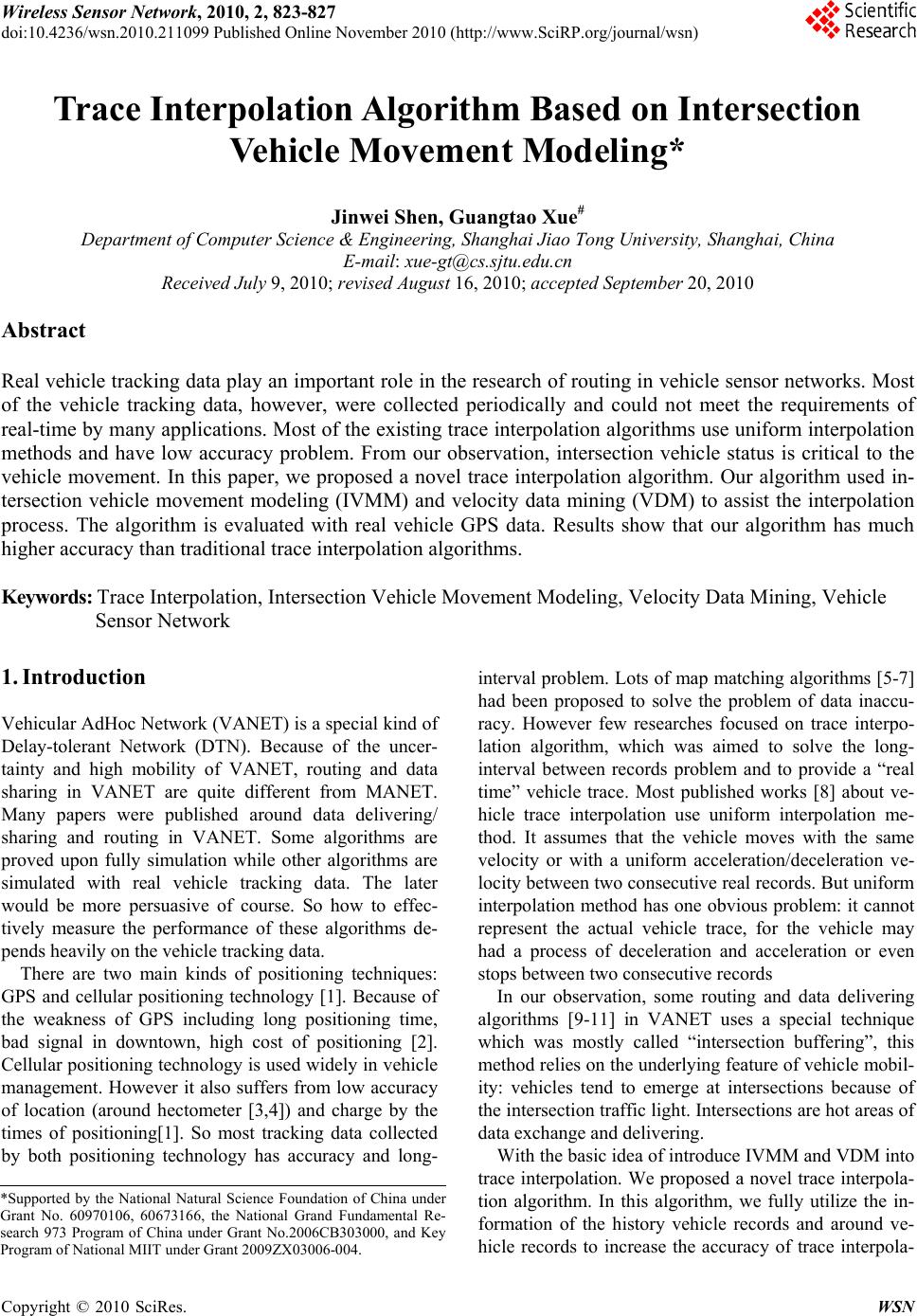Wireless Sensor Network, 2010, 2, 823-827
doi:10.4236/wsn.2010.211099 Published Online November 2010 (http://www.SciRP.org/journal/wsn)
Trace Interpolation Algorithm Based on Intersection
Vehicle Movement Modeling*
Jinwei Shen, Guangtao Xue#
Department of Computer Science & Engineering, Shanghai Jiao Tong University, Shanghai, China
Received July 9, 2010; revised August 16, 2010; accepted September 20, 2010
Abstract
Real vehicle tracking data play an important role in the research of routing in vehicle sensor networks. Most
of the vehicle tracking data, however, were collected periodically and could not meet the requirements of
real-time by many applications. Most of the existing trace interpolation algorithms use uniform interpolation
methods and have low accuracy problem. From our observation, intersection vehicle status is critical to the
vehicle movement. In this paper, we proposed a novel trace interpolation algorithm. Our algorithm used in-
tersection vehicle movement modeling (IVMM) and velocity data mining (VDM) to assist the interpolation
process. The algorithm is evaluated with real vehicle GPS data. Results show that our algorithm has much
higher accuracy than traditional trace interpolation algorithms.
Keywords: Trace Interpolation, Intersection Vehicle Movement Modeling, Velocity Data Mining, Vehicle
Sensor Network
1. Introduction
Vehicular AdHoc Network (VANET) is a special kind of
Delay-tolerant Network (DTN). Because of the uncer-
tainty and high mobility of VANET, routing and data
sharing in VANET are quite different from MANET.
Many papers were published around data delivering/
sharing and routing in VANET. Some algorithms are
proved upon fully simulation while other algorithms are
simulated with real vehicle tracking data. The later
would be more persuasive of course. So how to effec-
tively measure the performance of these algorithms de-
pends heavily on the vehicle tracking data.
There are two main kinds of positioning techniques:
GPS and cellular positioning technology [1]. Because of
the weakness of GPS including long positioning time,
bad signal in downtown, high cost of positioning [2].
Cellular positioning technolog y is used widely in vehicle
management. However it also suffers from low accuracy
of location (around hectometer [3,4]) and charge by the
times of positioning[1]. So most tracking data collected
by both positioning technology has accuracy and long-
interval problem. Lots of map matching algorithms [5-7]
had been proposed to solve the problem of data inaccu-
racy. However few researches focused on trace interpo-
lation algorithm, which was aimed to solve the long-
interval between records problem and to provide a “real
time” vehicle trace. Most published works [8] about ve-
hicle trace interpolation use uniform interpolation me-
thod. It assumes that the vehicle moves with the same
velocity or with a uniform acceleration/deceleration ve-
locity between two consecutive real reco rds. But uniform
interpolation method has one obvious problem: it cannot
represent the actual vehicle trace, for the vehicle may
had a process of deceleration and acceleration or even
stops between two consecutive records
In our observation, some routing and data delivering
algorithms [9-11] in VANET uses a special technique
which was mostly called “intersection buffering”, this
method relies on the underlying feature of vehicle mobil-
ity: vehicles tend to emerge at intersections because of
the intersection traffic light. Intersections are hot areas of
data exchange and delivering.
With the basic idea of introduce IVMM and VDM into
trace interpolation. We proposed a novel trace interpola-
tion algorithm. In this algorithm, we fully utilize the in-
formation of the history vehicle records and around ve-
hicle records to increase the accuracy of trace interpola-
*Supported by the National Natural Science Foundation of China unde
r
Grant No. 60970106, 60673166, the National Grand Fundamental Re-
search 973 Program of China under Grant No.2006CB303000, and Key
Program o f Na t i o nal MIIT under Grant 2009ZX03 0 0 6 -004.

J. W. SHEN ET AL.
824
tion algorithm.
The rest of this paper is organized as follows. In Sec-
tion 2, we introduce the IVMM and VDM technique and
our trace interpolation algorithm. Section 3 provides the
experimental results based on real tracking data. Section
4 includes the conclusion of this paper.
2. Trace Interpolation Algorithm
This paper’s work is based on data collected by 4000
taxis in Shanghai urban setting during several months in
2006, and we have the digital map information of the
whole area. Every record in the dataset includes the ve-
hicle’s id, vehicle’s GPS position, velocity information,
vehicle direction and timestamp. The interval of the
records varies from seconds to minutes.
Table 1 presents us two consecutive vehicle tracking
records with some fields omitted.
Since map matching is not what we concerned in this
paper, we assume that record r1 was matched to road
position p1 on road C1C2 and record r2 was matched to
position p2 on road C3C4, and the vehicle drives from p1
to p2 through cross C2 and C3 as depicted in Figure 1.
Suppose t1 and t2 has a gap of 1 min, if the required
timestamp granularity by application is 1 sec, then trace
interpolation is used to get the records or to find out
where the vehicle is at each second between t1 and t2. If
we know how fast the vehicle drives at each position
along the matched roads, it will be easy for us to know
where the vehicle is at timestamp tx. So trace interpola-
tion problem could be mapped to velocity finding prob-
lem.
In uniform interpolation algorithm, uniform velocity
distribution was adopted, which means during the time t1
Table.1 Two vehicle records.
Figure 1. Map matched vehicle records.
to t2 the velocity of the vehicle is calculated by
1223322 1
()/()VpCCCCptt

 . This could hardly
match the real case.
Following introduces our trace replay algorithm:
2.1. Intersection Vehicle Movement Modeling
Traditional interpolate algorithm assumes the vehicle
move through the intersections at its normal speed with-
out deceleration and stop. In reality, vehicles rarely keep
the normal speed at the intersection because of traffic
control signals [11]. Most vehicles experience decelera-
tion and acceleration and often wait in line with full stop
[12].
There are many different intersection structures in re-
ality, such as signalized, isolated, roundabout, etc. Our
intersection velocity model only studies the vehicle move-
ment at the signalized intersection with two crossing
paths. However different intersections would still have
different traffic light models, and it is hard to precisely
build different intersection models to different intersec-
tions for we don’t have the traffic light information for
each intersection. What’s more, a precise intersection
model requires a relatively high volume of traffic density.
We did some analysis based on the dataset and found
there’s an average of 10 vehicle records near one inter-
section per 2 min. With this observation, we compro-
mised to build a simplified intersection model for all the
signalized intersections. In this model, we had a simpli-
fied traffic light model: (1) turn to right is always per-
mitted (2) one of the two directions is fully permitted to
go any direction at a time, and we assume the queue of
vehicles would not surpass a specified length, which
means the vehicle would not stop at a po sition that is far
away from an intersection.
Since most vehicles experience deceleration and acce-
leration and sometimes wait in line with full stop, in our
simplified model, we divide the intersection vehicle ve-
locity model into two categories. As shown in Figure 2.
The first one has a full stop while the second one ju st has
a slight deceleration and acceleration.
When a vehicle’s two consecutive records matched on
two different roads, the interpolated trace between them
would get through intersection. Our task is to find out th e
intersection status of Ci at any time tx. Thus we will be
able to distinguish if a vehicle stops at the intersection Ci
at time tx and how long it stops if it did stops.
We utilize a voting mechanism to decide the status
1,
0,
i
verticaldirection green
Sverticaldirection red


 of an intersection Ci at
time tx.
First we find the involved (time-space close) record
Record
name x y Velocity Timestamp
r1 121.467 31.2195 v1 t
1
r2 121.469 31.2166 v2 t
2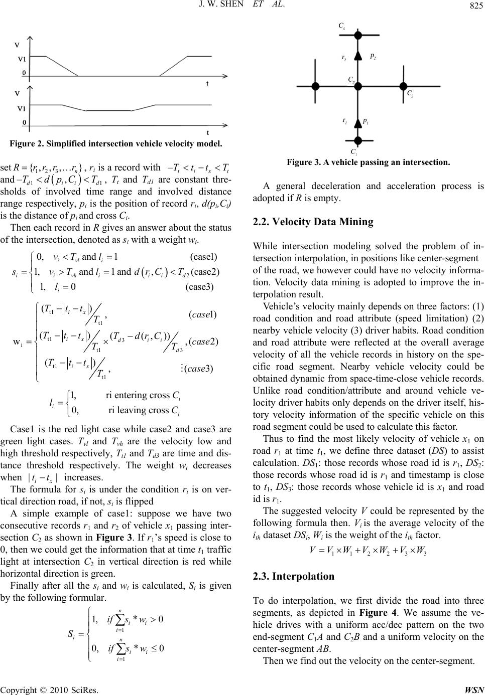

J. W. SHEN ET AL.
825
Figure 2. Simplified intersection vehicle velocity model.
set 123 {,, ,}
n
Rrrr r, ri is a record with –tix t TttT
and 

11
–,
diid
TdpCT
, Tt and Td1 are constant thre-
sholds of involved time range and involved distance
range respectively, pi is the position of record ri, d(pi,Ci)
is the distance of pi and cross Ci.
Then ea ch recor d in R give s an an sw er ab out th e s tatu s
of the intersection, denoted as si with a weight wi.

2
0,and 1(case1)
1,and1and ,(case2)
1,0(case3)
ivl i
iivhi iid
i
vT l
svTl drCT
l



 



t1
t1
t1 3
it1 3
t1
t1
()
,(1)
()
((,))
w,(2)
()
,(3)
ix
ix dii
d
ix
Tttcase
T
TttTdrCcase
TT
Ttt case
T











1,ri entering cross
0,ri leaving cross
i
ii
C
lC



Case1 is the red light case while case2 and case3 are
green light cases. Tvl and Tvh are the velocity low and
high threshold respectively, Tt1 and Td3 are time and dis-
tance threshold respectively. The weight wi decreases
when ||
ix
tt increases.
The formula for si is under the condition ri is on ver-
tical direction road, if not, si is flipped
A simple example of case1: suppose we have two
consecutive records r1 and r2 of vehicle x1 passing inter-
section C2 as shown in Figure 3. If r1’s speed is close to
0, then we could get the info rmation that at ti me t1 traffic
light at intersection C2 in vertical direction is red while
horizontal direction is green.
Finally after all the si and wi is calculated, Si is given
by the following formular.
1
1
1,* 0
0,* 0
n
ii
i
in
ii
i
ifs w
S
ifs w











Figure 3. A vehicle passing an intersection.
A general deceleration and acceleration process is
adopted if R is empty.
2.2. Velocity Data Mining
While intersection modeling solved the problem of in-
tersection interpolation, in positions like center-segment
of the road, we however could have no velocity informa-
tion. Velocity data mining is adopted to improve the in-
terpolation result.
Vehicle’s velocity mainly depends on three facto rs: (1)
road condition and road attribute (speed limitation) (2)
nearby vehicle velocity (3) driver habits. Road condition
and road attribute were reflected at the overall average
velocity of all the vehicle records in history on the spe-
cific road segment. Nearby vehicle velocity could be
obtained dynamic from space-time-close vehicle records.
Unlike road condition/attribute and around vehicle ve-
locity driver habits only de pends on the driver itself, his-
tory velocity information of the specific vehicle on this
road segment could be used to calculate this factor.
Thus to find the most likely velocity of vehicle x1 on
road r1 at time t1, we define three dataset (DS) to assist
calculation. DS1: those records whose road id is r1, DS2:
those records whose road id is r1 and timestamp is close
to t1, DS3: those records whose vehicle id is x1 and road
id is r1.
The suggested velocity V could be represented by the
following formula then. Vi is the average velocity of the
ith dataset DSi, Wi is the weight of the ith factor.
112 233
VVWVWVW




2.3. Interpolation
To do interpolation, we first divide the road into three
segments, as depicted in Figure 4. We assume the ve-
hicle drives with a uniform acc/dec pattern on the two
end-segment C1A and C2B and a uniform velocity on the
center-segment AB.
Then we find out the velocity on the center-segment.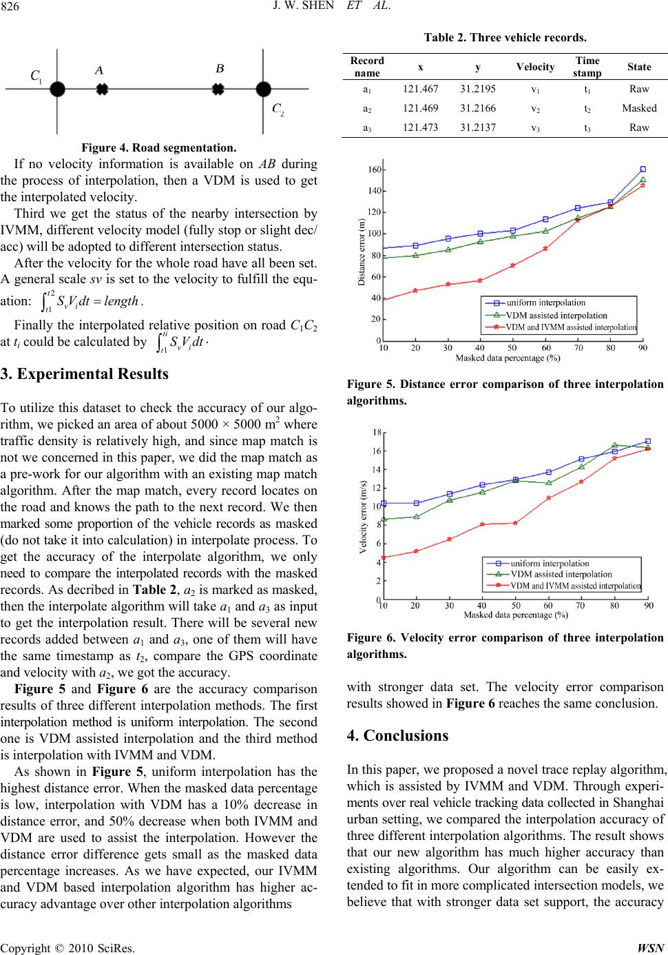

J. W. SHEN ET AL.
826
Figure 4. Road segmentation.
If no velocity information is available on AB during
the process of interpolation, then a VDM is used to get
the interpolated velocity.
Third we get the status of the nearby intersection by
IVMM, different velocity model (fully stop or slight dec/
acc) will be adopted to different intersection status.
After the velocity for the whole road have all been set.
A general scale sv is set to the velocity to fulfill th e equ-
ation: 2
1
t
vi
tSV dtlength
.
Finally the interpolated relative position on road C1C2
at ti could be calculated by 1
ti
vi
tSVdt

3. Experimental Results
To utilize this dataset to check the accuracy of our algo-
rithm, we picked an area of abou t 5000 × 5000 m2 where
traffic density is relatively high, and since map match is
not we concerned in this paper, we did the map match as
a pre-work for our algorithm with an existing map match
algorithm. After the map match, every record locates on
the road and knows the path to the next record. We then
marked some proportion of the vehicle records as masked
(do not take it into calculatio n) in interpolate process. To
get the accuracy of the interpolate algorithm, we only
need to compare the interpolated records with the masked
records. As decribed in Table 2, a2 is marked as masked,
then the interpolate algo rithm will take a1 and a3 as input
to get the interpolation result. There will be several new
records added between a1 and a3, one of them will have
the same timestamp as t2, compare the GPS coordinate
and velocity with a2, we got the accuracy.
Figure 5 and Figure 6 are the accuracy comparison
results of three different interpolation methods. The first
interpolation method is uniform interpolation. The second
one is VDM assisted interpolation and the third method
is interpolation with IVMM and VDM.
As shown in Figure 5, uniform interpolation has the
highest distance error. When the masked data percentage
is low, interpolation with VDM has a 10% decrease in
distance error, and 50% decrease when both IVMM and
VDM are used to assist the interpolation. However the
distance error difference gets small as the masked data
percentage increases. As we have expected, our IVMM
and VDM based interpolation algorithm has higher ac-
curacy advantage over other interpolation algorithms
Table 2. Three vehicle records.
Figure 5. Distance error comparison of three interpolation
algorithms.
Figure 6. Velocity error comparison of three interpolation
algorithms.
with stronger data set. The velocity error comparison
results showed in Figure 6 reaches the same conclusion.
4. Conclusions
In this paper, we proposed a novel trace replay algorithm,
which is assisted by IVMM and VDM. Through experi-
ments over real vehicle tracking data collected in Sha ng ha i
urban setting, we compared the interpolation accuracy of
three different interpolation algorithms. The result shows
that our new algorithm has much higher accuracy than
existing algorithms. Our algorithm can be easily ex-
tended to fit in more complicated intersection models, we
believe that with stronger data set support, the accuracy
Record
name x y Velocity
Time
stamp State
a1 121.467 31.2195 v1 t
1 Raw
a2 121.469 31.2166 v2 t
2 Masked
a3 121.473 31.2137 v3 t
3 Raw

J. W. SHEN ET AL.
827
of our algorithm can be even higher.
5. References
[1] X. W. Chen, F. Z. Zhang, M. Sun and Y. H. Luo, “Sys-
tem Architecture of LBS Based on Spatial Information
Integration,” IEEE International conference on Geos-
cience and Remote Sensing Symposium, 2004. IGARSS
'04. Proceedings, Anchorage, Alaska, Vol. 4, September
2004, pp. 2409-2411.
[2] Y. Q. Huang and X. M. Gu, “The Combination of GPS
and GSM Mobile Location Technology,” Journal of
Jiamusi University, Sicence, Vol. 23, October 2005, pp.
530-533.
[3] L. Perusco and K. Michael, “Humancentric Applications
of Precise Location Based Services,” IEEE International
Conference on e-Business Engineering, Beijing, 18-21
October 2005, pp. 409-418.
[4] M. Wallbaum and S. Diepolder, “Benchmarking Wireless
Location Systems,” The Second International Workshop
on Mobile Commerce and Services, IEEE, Germany, July
2005, pp. 42-51.
[5] D. Bernstein and A. Kornhauser, “An Introduction to
Map Matching for Personal Navigation Assistants,” Tech-
nical report, New Jersey TIDE Center Technical Report,
1996.
[6] M. Quddus, W. Ochieng, L. Zhao and R. Noland, “A
General Map Matching Algorithm for Transport Tele-
matics Applications,” GPS Solutions Journal, Vol. 7, No.
3, 2003, pp. 157-167.
[7] H. Yin and O. Wolfson, “A Weight-Based Map Matching
Method in Moving Objects Databases,” In Proceedings of
16th SSDBM conference, Santorini Island, Greece, 2004,
pp. 437-438.
[8] H. H. Gao, K. B. Jia, X. H. Bao and J. He, “Research and
Implementation of Road Match and Trace Replay Algo-
rithm,” MultiMedia and Information Technology, Three
Gorges, 30-31 December 2008, pp. 74-77.
[9] J. Zhao and G. Cao, “VADD: Vehicle-Assisted Data
Delivery in Vehicular Ad Hoc Networks,” Proceedings of
IEEE INFOCOM’06, Barcelona, April 2006, pp. 1-12.
[10] M. Jerbi, S. M. Senouci, R. Meraihi and Y. Ghamri-
Doudane, “An Improved Vehicular Ad Hoc Routing Pro-
tocol for City Environments,” IEEE International Confe-
rence on Communications, Glasgow, 24-28 June 2007, pp.
3972-3979.
[11] J. Zhao, Y. Zhang and G. Cao, “Data Pouring and Buf-
fering on the Road: A New Data Disseminat ion Paradigm
for Vehicular Ad Hoc Networks,” IEEE Transactions on
Vehicular Technology, Vol. 56, No. 6, November 2007,
pp. 3266-3277.
[12] F. Dion, H. Rakha and Y. Kang, “Comparison of Delay
Estimates at Undersaturated and Over-Saturated Pre-
Timed Signalized Intersections,” Transportation Research,
Part B: Methodological, Vol. 38, No. 2, Feburary 2004,
pp. 99-122.