Journal of Modern Physics, 2013, 4, 70-93
http://dx.doi.org/10.4236/jmp.2013.44A010 Published Online April 2013 (http://www.scirp.org/journal/jmp)
Predicting the Binding Energies of the 1s Nuclides with
High Precision, Based on Baryons which Are Yang-Mills
Magnetic Monopoles
Jay R. Yablon
Schenectady, New York, USA
Received March 22, 2013; revised April 24, 2013; accepted April 29, 2013
Copyright © 2013 Jay R. Yablon. This is an open access article distributed under the Creative Commons Attribution License, which
permits unrestricted use, distribution, and reproduction in any medium, provided the original work is properly cited.
ABSTRACT
In an earlier paper, the author employed the thesis that baryons are Yang-Mills magnetic monopoles and that proton and
neutron binding energies are determined based on their up and down current quark masses to predict a relationship
among the electron and up and down quark masses within experimental errors and to obtain a very accurate relationship
for nuclear binding energies generally and for the binding of 56Fe in particular. The free proton and neutron were under-
stood to each contain intrinsic binding energies which confine their quarks, wherein some or most (never all) of this
energy is released for binding when they are fused into composite nuclides. The purpose of this paper is to further ad-
vance this thesis by seeing whether it can explain the specific empirical binding energies of the light 1s nuclides,
namely, 2H, 3H, 3He and 4He, with high precision. As the method to achieve this, we show how these 1s binding ener-
gies are in fact the components of inner and outer tensor products of Yang-Mills matrices which are implicit in the ex-
pressions for these intrinsic binding energies. The result is that the binding energies for the 4He, 3He and 3H nucleons
are respectively, independently, explained to less than four parts in one million, four parts in 100,000, and seven parts in
one million, all in AMU. Further, we are able to exactly relate the neutron minus proton mass difference to a function of
the up and down current quark masses, which in turn enables us to explain the 2H binding energy most precisely of all,
to just over 8 parts in ten million. These energies have never before been theoretically explained with such accuracy,
which leads to the conclusion that the underlying thesis provides the strongest theoretical explanation to date of what
baryons are, and of how protons and neutrons confine their quarks and bind together into composite nuclides. As is also
reviewed in Section 9, these results may lay the foundation for more easily catalyzing nuclear fusion energy release.
Keywords: Nuclides; Binding Energy; Deuteron; Triton; Helion; Alpha; Alpha Decay; Beta Decay; Yang-Mills;
Magnetic Monopoles; Solar Fusion; Nuclear Fusion; Confinement
1. Introduction: Summary Review of the
Thesis that Baryons Are Yang-Mills
Magnetic Monopoles with Binding
Energies Based on Their Current Quark
Masses
In an earlier paper [1], the author developed the thesis
that magnetic monopole densities which come into exis-
tence in a non-Abelian Yang-Mills gauge theory of
non-commuting vector gauge boson fielG
ds

are
synonymous with baryon densities. That is, baryons, in-
cluding the protons and neutrons which form the vast
preponderance of matter in the universe, are Yang-Mills
magnetic monopoles. Conversely, magnetic monopoles,
long pursued since the time of Maxwell, have always
been hiding in plain sight, in Yang-Mills incarnation, as
baryons, and especially, as protons and neutrons.
Maxwell’s equations themselves provide the theoreti-
cal foundation for this thesis, because if one starts with
the classical electric charge and magnetic monopole field
equations (respectively, (2.1) and (2.2) of [1]):

[]
JF DG
g
DDG
 

 


 

PFFF
(1.1)

 
 (1.2)


DiG


  and combines the magnetic charge
Equation (1.2) with a Yang-Mills (non-Abelian) field
strength tensor

is an N × N ma-


which, like G
F
C
opyright © 2013 SciRes. JMP

J. R. YABLON 71
trix for a simple gauge group SU(N) ((2.3) of [1]):
[]
,
F
GG
DG DG
 
 
 

iGG
D G
 
 



,,
G
GG
 


G
(1.3)
one immediately comes upon the non-vanishing mag-
netic monopole ((2.4) of [1]):

,PiG
GG
 


 

 

(1.4)
The question then becomes whether such magnetic
monopoles (1.4) actually do exist in the material universe,
and if so, in what form. The thesis developed in [1] is not
only that these magnetic monopoles do exist, but that
they permeate the material universe in the form of bary-
ons, especially as the protons and neutrons observed
everywhere and anywhere that matter exists.
Of course, t’Hooft [2] and Polyakov [3] realized sev-
eral decades ago that non-Abelian gauge theories lead to
non-vanishing magnetic monopoles. But their monopoles
have very high energies which make them not suitable
for being baryons such as protons and neutrons. Follow-
ing t’Hooft, the author in [1] does make use of the
t’Hooft monopole Lagrangian from (2.1) of [2] to calcu-
late the energies of these magnetic monopoles (1.4). But
whereas t’Hooft introduces an ansatz about the radial
behavior of the gauge bosons

, the author instead
makes use of a Gaussian ansatz borrowed from Equation
(14) of Ohanian’s [4] for the radial behavior of fermions.
Moreover, the fermions for which this ansatz is em-
ployed enter on the very solid foundation of taking the
inverse GIJ


of Maxell’s charge Equation (1.1)
(essentially calculating the configuration space inverse


1
D
 

gD


), and then combining this with the
relationship J


 
0J

that emerges from satisfying
the charge conservation (continuity) equation



in Dirac theory. Specifically, it was found that in the
low-perturbation limit, magnetic monopoles (1.4) can be
re-expressed as a three-fermion system ((3.12) of [1]):
 
 
 
 
 
 
11
11
22
22
2""
""
Pm

 


 

 



 


33
33
""mm

 







 

(1.5)
Above,

i;1,2,3i

 are three distinct Dirac spinor
wavefunctions which emerge following three distinct
substitutions of GI
  
J I


 
 
""
ii
m
—which cap-
tures the inverse of Maxwell’s charge Equation (1.1)
combined with Dirac theory—into the (1.4) magnetic
monopole which utilizes the Yang-Mills field strength
(1.3) in combination with Maxwell’s magnetic monopole
Equation (1.2). The detailed derivation of (1.5) from (1.4)
also makes use of Sections 6.2, 6.14 and 5.5 of [5] per-
taining to Compton scattering and the fermion com-
pleteness relation, and carefully accounts for mass de-
grees of freedom as between fermions and bosons. The
quoted denominators


 and “quasi commuta-
tors” 2
i
 





 in the above make use of a


compact notation developed and explained in Section 3
of [1], see specifically (3.9) and (3.10) therein.
Then, via Fermi-Dirac Exclusion, the author employed
the QCD color group SU (3)C to require that each of the
three

i

be SU(3 )C vectors in distinct quantum color
eigenstates R, G, B, which then leads in (5.5) of [1] to a
magnetic monopole:
Tr2 ""
""""
RR
RR
GG BB
GG BB
Pm
mm

 
 

 

  




 


 (1.6)

 



This is similar to (1.5) but for the emergence of the
trace. Associating each color with the spacetime index in
the related


operator, i.e., ,RG
  B and



,
and keeping in mind that Tr P


RGB
is antisymmetric in
all spacetime indexes, we express this antisymmetry with
wedge products as


 
P
. So the natu-
ral antisymmetry of a magnetic monopole


leads
straight to the required antisymmetric color singlet
wavefunction






,,,RGB GBRBRG
P
for a baryon.
Indeed, in hindsight, this antisymmetry together with
three vector indexes to accommodate three vector current
densities and the three additive terms in the


of
(1.2) should have been a tip-off that magnetic monopoles
would naturally make good baryons. Further, upon inte-
gration over a closed surface via Gauss’/Stokes’ theorem,
magnetic monopole (1.6) is shown to emit and absorb
color singlets with the symmetric color wavefunction
RR

GG BB
logical stability of these magnetic monopoles was estab-
expected of a meson. And, in Section 1
of [1], it was shown how magnetic monopoles naturally
contain their gauge fields in non-Abelian gauge theory
via the differential forms relationship dd = 0 for precisely
the same reasons rooted in spacetime geometry that
magnetic monopoles do not exist at all in Abelian gauge
theory. Thus, QCD itself deductively emerges from the
thesis that baryons are Yang-Mills magnetic monopoles,
and we began to associate monopole (1.6) with a baryon.
It was then shown in Sections 6 through 8 of [1] that
these SU(3) monopoles may be made topologically stable
by symmetry breaking from larger SU(4) gauge groups
which yield the baryon and electric charge quantum
numbers of a proton and neutron. Specifically, the topo-

J. R. YABLON 72
lished in Sections 6 and 8 of [1] based on Cheng and Li
[6] at 472-473 and Weinberg [7] at 442. The proton and
neutron are developed as particular types of magnetic
monopole in Section 7 of [1] making use of SU(4) gauge
groups for baryon minus lepton number BL based on
Volovok’s [8], Section 12.2.2. The spons symme-
try breaking of these SU(4) gauge groups is then fash-
ioned on Georgi-Glashow’s SU(5) GUT model [9] re-
viewed in detail in Section 8 of [1].
By then employing the earlier-r
taneou
eferenced “Gaussian
ansatz” from Ohanian’s [4], namely ((9.9) of [1]):
 


2
31rr
 0
24
2
πexp2 rup 




 (1.7)
for the radial behavior of the fermion wavefunctions,
of [1], the author
us
ner
together with the t’Hooft monopole Lagrangian from (2.1)
of [2] (see (9.2) of [1]) it became possible to analytically
calculate the energies of these Yang-Mills magnetic
monopoles (1.6) following their development into topo-
logically stable protons and neutrons.
Specifically, in Sections 11 and 12
ed the pure gauge field terms gauge
L of the t’Hooft
monopole Lagrangian to specify the egy of the Yang-
Mills magnetic monopoles, exclusive of the vacuum

,
via (11.7) of [1]:
3
gauge
1
dT
2
Ex 
 
L3 r d FFx

  . (1.8)
We then made use in (1.8) of field strength tensors for
protons and neutrons developed via Gauss’/Stokes’ the-
orem from (1.6) in (11.3) and (11.4) of [1], respectively:
P
Tr
2
""
dd
dd ""
uu
uu
imm
 
 



 
 






(1.9)
F


N
Tr
2
""
uu
uu
F
im


 











" "
dd
dd
m












(1.10)
u
where

and d

are Dirac wavefunctions for up and
uar de
ectron mass
is
 
down qks, toduce three relationships which yielded
remarkable concurrence with empirical data.
First, we found in (11.22) of [1] that the el
related to up and down quark masses according to:
3
2
2π
u
m, (1.11)
whervisor

0.510998928 MeV3
ed
mm
e the di
3
2
2π results as a natural conse-
dimenquence of the three-sional integration (1.8) when
the Gaussian ansatz for fermions is specified as in (1.7),
and where the wavelengths in (1.7) are taken to be re-
lated to the quark masses via the de Broglie relation
mc

 .
aSecondnd third, we found in (12.12) and (12.13) of
[1] that if one postulates the current mass of the up quark
to be equal to the deuteron (2H nucleus) binding energy
based on 1) empirical concurrence within experimental
errors and 2) regarding nucleons to be resonant cavities
with binding energies determined in relation to their up
and down current quark masses, then the proton and neu-
tron each possess respective intrinsic, latent binding en-
ergies B (i.e., energies intrinsically available for nuclear
binding):


3
2
P
B244 2π
7.640679 MeV
ud dudu
mm mmmm 

(1.12)


3
2
N
B244 2π
9.812358 MeV
du uudd
mm mmmm 

(1.13)
So for a nucleus with an equal number of protons and
neutrons, the average binding energy per nucleon is pre-
dicted to be 8.726519 MeV. Not only does this explain
why a typical nucleus beyond the very lightest (which we
shall be studying in detail here) has a binding energy in
exactly this vicinity (see Figure 1 below), but when this
is applied to 56Fe with 26 protons and 30 neutrons—
which has the distinction of using a higher percentage of
this available binding energy than any other nuclide—we
see that the latent available binding energy is predicted
to be ((12.14) of [1]):


56
B Fe267.640679 MeV
309.812358 MeV
493.028394 MeV



(1.14)
This contrasts remarkably with the observed 56Fe
bi
resonant
ca
nding energy of 492.253892 MeV. That is, precisely
99.8429093% of the available binding energy predicted
by this model of nucleons as Yang-Mills magnetic mono-
poles goes into binding together the 56Fe nucleus, with a
small 0.1570907% balance reserved for confining quarks
within each nucleon. This means while quarks are very
much freer in the nucleons of 56Fe than in free nucleons
(which also appears to explain the “first EMC effect”
[10]), their confinement is never fully overcome. Con-
finement bends but never breaks. Quarks step back from
the brink of becoming de-confined in 56Fe as one moves
to even heavier nuclides, and remain confined no matter
what the nuclide. Iron-56 thus sits at the theoretical
crossroads of fission, fusion and confinement.
This thesis that protons and neutrons are
vities which emit and absorb energies that directly
manifest their current quark masses will be central to the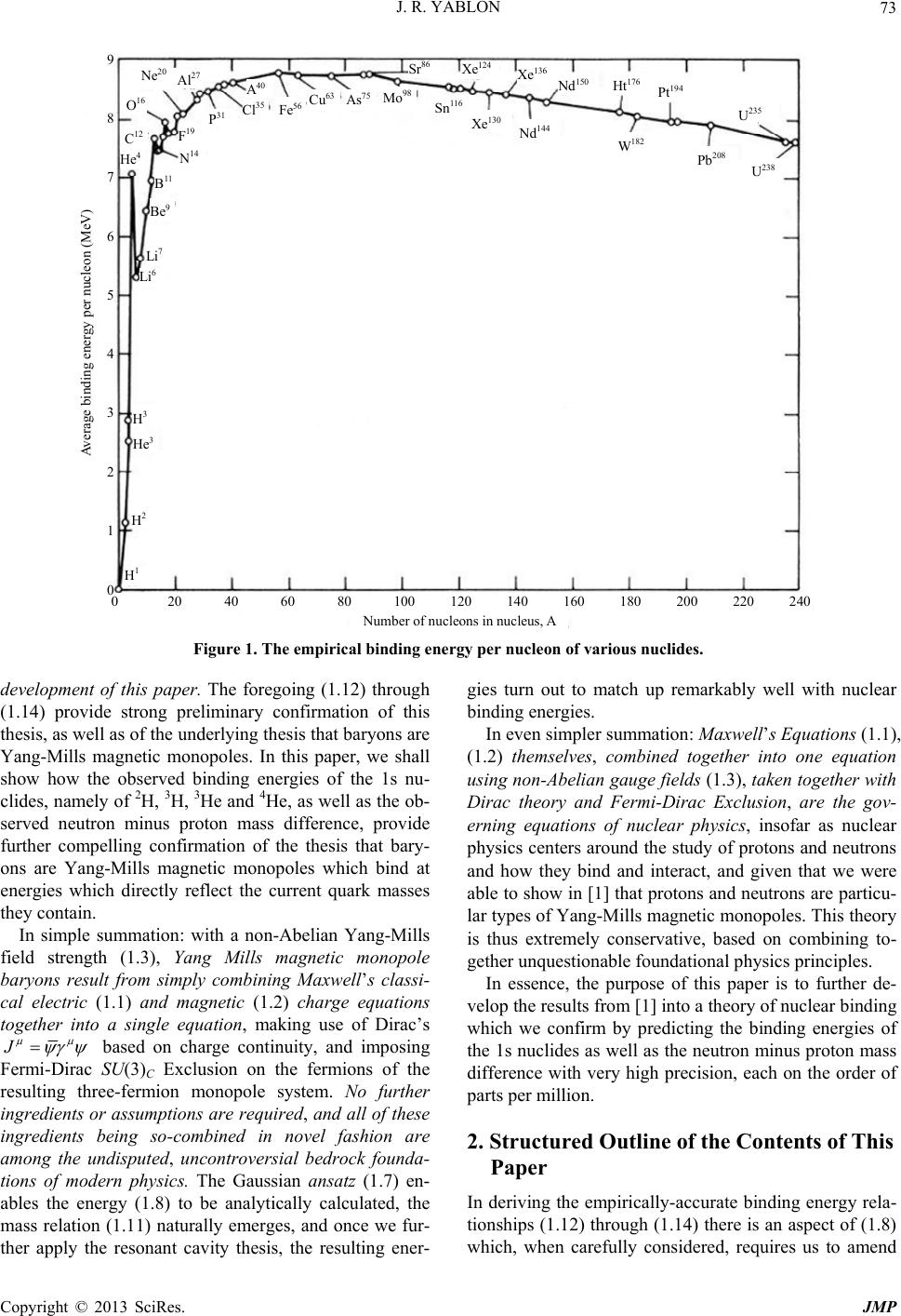

J. R. YABLON 73
N
e
20
0 20 40 60 80 100 120 140 160 180 200 220 240
9
Number of nucleons in nucleus
,
A
8
7
6
5
4
3
2
1
0
Average binding energy per nucleon (MeV)
Li
6
Li
7
H
1
H
2
He
3
H
3
He
4
Be
9
B
11
N
14
F
19
P
31
C
12
O
16
Al
27
Cl
35
A
40
Fe
56
Cu
63
As
75
Mo
98
Xe
130
N
d
144
W
182
Sn
116
Pb
208
U
238
U
235
Pt
194 Ht
176
N
d
150
Xe
136 Xe
124
Sr
86
Figure 1. The empirical binding ener gy per nuc leon of various nuclides.
evelopment of this paper. The foregoing (1.12) through
ummation: with a non-Abelian Yang-Mills
fie
d
(1.14) provide strong preliminary confirmation of this
thesis, as well as of the underlying thesis that baryons are
Yang-Mills magnetic monopoles. In this paper, we shall
show how the observed binding energies of the 1s nu-
clides, namely of 2H, 3H, 3He and 4He, as well as the ob-
served neutron minus proton mass difference, provide
further compelling confirmation of the thesis that bary-
ons are Yang-Mills magnetic monopoles which bind at
energies which directly reflect the current quark masses
they contain.
In simple s
ld strength (1.3), Yang Mills magnetic monopole
baryons result from simply combining Maxwell’s classi-
cal electric (1.1) and magnetic (1.2) charge equations
together into a single equation, making use of Dirac’s
J


  based on charge continuity, and imposing
SU(3)C Exclusion on the fermions of the
resulting three-fermion monopole system. No further
ingredients or assumptions are required, and all of these
ingredients being so-combined in novel fashion are
among the undisputed, uncontroversial bedrock founda-
tions of modern physics. The Gaussian ansatz (1.7) en-
ables the energy (1.8) to be analytically calculated, the
mass relation (1.11) naturally emerges, and once we fur-
ther apply the resonant cavity thesis, the resulting ener-
binding energies.
In even simpler summation: Maxwell’s Equations (1.1),
(1.2) themselves,
Fermi-Dirac
gies turn out to match up remarkably well with nuclear
combined together into one equation
us
g
w
utline of the Contents of This
tio .12) through (1.14) there is an aspect of (1.8)
ing non-Abelian gauge fields (1.3), taken together with
Dirac theory and Fermi-Dirac Exclusion, are the gov-
erning equations of nuclear physics, insofar as nuclear
physics centers around the study of protons and neutrons
and how they bind and interact, and given that we were
able to show in [1] that protons and neutrons are particu-
lar types of Yang-Mills magnetic monopoles. This theory
is thus extremely conservative, based on combining to-
gether unquestionable foundational physics principles.
In essence, the purpose of this paper is to further de-
velop the results from [1] into a theory of nuclear bindin
hich we confirm by predicting the binding energies of
the 1s nuclides as well as the neutron minus proton mass
difference with very high precision, each on the order of
parts per million.
2. Structured O
Paper
In deriving the empirically-accurate binding energy rela-
nships (1
which, when carefully considered, requires us to amend

J. R. YABLON 74
the Lagrangian in (1.8) in a slight but important way.
This amendment, developed in Section 3, will reveal that
the latent binding energies (1.12) and (1.13) actually em-
ploy the inner and outer tensor products of two 3 × 3
SU(3) matrices, one for protons, and one for neutrons.
These matrices, and their inner and outer products, will
be critical to the methodological development thereafter.
In section 4 we lay the foundation for being able to de-
rive the binding energies of the 1s nuclides using the
ea
or the 4He alpha
bi
parts in one million
A
ss excess rather
th
how these can be combined to ex-
pr
not only the
accuracy of the re
ical, because the
po
e results for 3H, 3He and
4H
y in Figure 11,
in
rlier-discussed postulate that the mass of the up quark
is equal to the deuteron (2H nucleus) binding energy, and
the thesis extrapolated from this that the binding energies
of nuclides generally are direct functions of the current
quark masses which their nucleons contain. Specifically,
in (4.9) through (4.11) infra, we develop two tensor outer
products and their components which will be critical in-
gredients for expressing 1s binding energies as functions
of up and down current quark masses.
Section 5 shows how this binding energy thesis leads
directly to a theoretical expression f
nding energy which matches empirical data to less than
3 parts in 1 million AMU. Exploring the meaning of this
result, we see that this binding energy together with that
of the 2H deuteron are actually components of a (3 × 3) ×
(3 × 3) fourth rank Yang Mills tensor of which the 2H
and 4He binding energies merely two samples. Thus, we
are motivated to think about binding energies generally
as components of Yang-Mills tensors. So the method for
characterizing binding energies is one of trying to match
up empirical binding energies with various expressions
which emerge from, or are components of, these Yang-
Mills tensors. In Section 6, we similarly obtain a theo-
retical expression for 3He helion binding to just under 4
parts in 100,000 AMU as well as its characterization in
terms of these Yang-Mills tensors.
Developing a similar expression for the 3H triton to
what ends up being just over three
MU turns out to be less straightforward than for any of
2H, 3He and 4He, and requires us to work with mass ex-
cess rather than binding energy. However, a bonus is that
in the process, we are also motivated to derive an expres-
sion for the neutron minus proton mass difference accu-
rate to just over 7 parts in ten million AMU. To maintain
clarity and focus on the underlying research ideas, these
results are summarized in Section 7, while their detailed
derivation is presented in the Appendix.
Section 8 aggregates the results of Sections 5 through
7, and couches them all in terms of ma
an binding energy. In this form, it becomes more
straightforward to study nuclear fusion processes involv-
ing these 1s nuclides.
Section 9 makes use of the mass excess results from
Section 8, and shows
ess the approximately 26.73 MeV of energy known to
be released during the solar fusion cycle 1
1
4H2e  
4
2He 2Energy
  entirely in terms of the up, down and
electron fermion masses. This highlights
sults for 2H, 3H, 3He and 4He binding
energies and the neutron minus proton mass difference,
but it establishes the approach one would use to do the
same for other types of nuclear fusion, and for fission
reactions. And, it vividly confirms the thesis that fusion
and fission and binding energies are directly based on the
masses of the quarks which are contained in protons and
neutrons, regarded as resonant cavities.
But perhaps the most important consequence of the
development in Section 9 is technolog
ssibility is developed via this “resonant cavity” analy-
sis that by bathing a store of hydrogen in gamma radia-
tion at certain specified, discrete frequencies which are
also defined functions of the up and down quark masses,
one can catalyze nuclear fusion and perhaps develop
more effective ways to practically exploit the promise of
nuclear fusion energy release.
In Section 10, we take a closer look at experimental
errors that still do reside in th
e binding and the neutron minus proton mass differ-
ence, generally at parts per 105, 106 or 107 AMU. We
explain why the original postulate identifying the up
quark mass exactly with the 2H deuteron binding energy
should be modified into the substitute postulate that the
theoretical neutron minus proton mass difference is an
exact relationship, and why the equality of the up quark
mass and the deuteron binding energy is simply a very
close approximation (to just over 8 parts in ten million)
rather than an exact relationship. We then are required to
adjust (recalibrate) all of the prior numeric mass and en-
ergy calculations accordingly, by about parts per million.
As a by-product, the up and down quark masses become
known with the same degree of experimental precision as
the electron rest mass and the neutron minus proton mass
difference, to ten decimal places in AMU.
Section 11 concludes by summarizing and consolidate-
ing these results, laying out most compactl
fra, how the thesis that baryons are Yang-Mills mag-
netic monopoles which fuse at binding energies reflective
of their current quark masses can be used to predict the
binding energies of the 4He alpha to less than four parts
in one million, of the 3He helion to less than four parts in
100,000, and of the 3H triton to less than seven parts in
one million, all in AMU. And of special import, by ex-
actly relating the neutron minus proton mass difference
to a function of the up and down quark masses, we are
enabled to predict the binding energy for the 2H deuteron
most precisely of all, to just over 8 parts in ten million.
What renders this work novel is 1) that the 1s light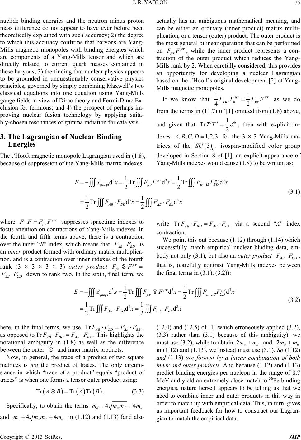

J. R. YABLON
© 2013 SciRes. JMP
75
in (1.8),
because of suppression of the Yang-Mills matrix indexes,
nuclide binding energies and the neutron minus protonactually has an ambiguous mathematical meaning, and
can be either an ordinary (inner product) matrix multi-
plication, or a tensor (outer) product. The outer product is
the most general bilinear operation that can be performed
on
mass difference do not appear to have ever before been
theoretically explained with such accuracy; 2) the degree
to which this accuracy confirms that baryons are Yang-
Mills magnetic monopoles with binding energies which
are components of a Yang-Mills tensor and which are
directly related to current quark masses contained in
these baryons; 3) the finding that nuclear physics appears
to be grounded in unquestionable conservative physics
principles, governed by simply combining Maxwell’s two
classical equations into one equation using Yang-Mills
gauge fields in view of Dirac theory and Fermi-Dirac Ex-
clusion for fermions; and 4) the prospect of perhaps im-
proving nuclear fusion technology by applying suita-
bly-chosen resonances of gamma radiation for catalysis.
3. The Lagrangian of Nuclear Binding
Energies

F
F


, while the inner product represents a con-
traction of the outer product which reduces the Yang-
Mills rank by 2. When carefully considered, this provides
an opportunity for developing a nuclear Lagrangian
based on the t’Hooft’s original development [2] of Yang-
Mills magnetic monopoles.
Copyright
The t’Hooft magnetic monopole Lagrangian used
If we know that 11
42
aa
F
FFF


 
 as we do
from the terms in (11.7) of [1] omitted from (1.8) above,
and given that 1
2
ij ij
TTTr


,,, 1,2,3ABCD
, then with explicit in-
dexes

for the 3 × 3 Yang-Mills ma-


3C SU

isospin-modified color group trices of the
developed in Section 8 of [1], an explicit appearance of
Yang-Mills indexes would cause (1.8) to be written as:
3
gauge
1
dTrExF 
 
L3 3
33
1
dTr d
22
11
Tr dd
22
AB BD
AB BDAB BA
FxFFx
FFxFF x
 
 



 
(3.1)
where
F
FFF



 suppresses spacetime indexes to
cus attention on contractions of Yang-Mills indexes. In
rth and fifth te
write TrAB BDAB BA
F
FFF

 via a second “A” index
contraction.
point this out because (
match empirical nuclear binding data, em-
bo
fo
the fourms above, there is a contraction
over the inner “B” index, which means that AB BD
F
F

is
an inn er product formed with ordinary matrix multiplica-
tion, and is a contraction over inner indexes ofrth
rank (3 × 3 × 3 × 3) outer product FF


We 1.12) through (1.14) which
successfully
dy not only (3.1), but also an outer product AB CD
F
F,
that is, (carefully contrast Yang-Mills indexes between
the fou


AB CD
F
F down to rank two. In the sixth, final term, we the final terms in (3.1), (3.2)):
3
gauge
1
dTrExF

 
 
L33
1
dTr d
AB CD
FxFFx
 


33
22
11
Tr d d
22
AB CDAA BB
FF xFF x


 
(3.2)
here, in the final terms, we use Tr AB CDAA BB
F
FFF,
s opposed toTr aAB BDAB BA
F
FFF. This highlights the
st
notational ambiguity in (1.8) as well as the difference
ter  and inner matr
ircum-
between the ouix products.
Now, in general, the trace of a product of two square
matrices is not the product of traces. The only c
ance in which “trace of a product” equals “product of
traces” is when one forms a tensor outer product using:



TrTr Tr
A
BAB . (3.3)
Specifically, to obtain the terms 44
udu
mmm
d
m
and 44
uudd
mmmm in (1.13) (and also
(12.4) and (12.5) of [1] which erroneously applied (3.2),
(3.3) rather than (3.1) because of this ambiguity), we
d
m and 2du mm st use (3.2), while to obtain 2u m mu

.13), we instead must uin (1.12) and (1
(1.13) are
se (3.1). So (1.12)
formed b
se matche binding
gian to match the empirical data.
and y a linear combination of both
inner and outer products. And because (1.12) and (1.13)
predict binding energies per nucleon in the range of 8.7
MeV and yield an extremely clo to 56F
energies, nature herself appears to be telling us that we
need to combine inner and outer products in this way in
order to match up with empirical data. This, in turn, gives
us important feedback for how to construct our Lagran-
(1.12) and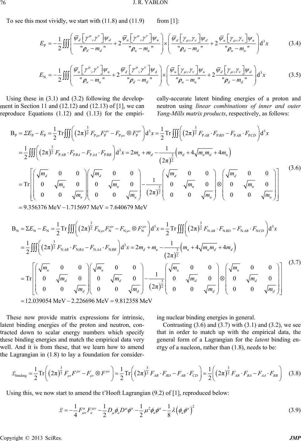

J. R. YABLON 76
To see this most vividly, we start with (11.8) and (11.9) from [1]:
3
"
u dduu  
 



 
 




P
12
2" ""
ddu
Emm
 




 
 

 



 2
d
""""
dduudd uu
x
mm







 
(3.4)
3
122d
"
uudd uudd
dd
E x
m
 
 
  

 


  
  


 




(3.5)
ment in Section 11 and (12.12) and (12.13) of [1], we can
produce Equations (1.12) and (1.13) for the empiri-
cally-accurate latent binding energies of
neutron using linear combinations of inner and outer
Yang-Mills matrix products, respectively, as follows:
N2" """" ""
uu dd uu
mm m  

 
 


Using these in (3.1) and (3.2) following the develop-
re
a proton and
 
 

33
22
PPP PPPPPPPP
11
BTr2πdTr2πd
22
μν μν
μν μνAB BDAB CD
ΣEEFFFFF FFFx
 
 
 
 
 
33
33
2PP PP 3
2
11
2πd2 4 4
22π
00 00
Tr0000
0000
AB BAAABBuddu du
dd
uu
uu
x
FFFFxmmmmmm
mm
mm
mm












3
2
00 00
10000
2π00 00
9.356376 MeV1.715697 MeV7.640679 MeV
dd
uu
uu
mm
mm
mm
 

  
  

    
  
 

 

(3.6)
 
 

33
33
22
NNNNNNNNN NN
33
2NN NN3
2
11
BTr2πdTr2πd
22
11
2πd24 4
22π
00 00
μν μν
μν μνABBDAB CD
ABBAAABBduuu dd
EEFFFFxFFFFx
FF FFxmmmmmm
mm
 
 
 
 





 

T r0000
0000
uu
dd
dd
mm
mm






3
2
100
2π00
12.039054 MeV2.226696 MeV9.812358 MeV
uu



 
 



These now provide matrix expressions for intrinsic,
latent binding energies of the proton and neutron, con-
00 00
00
00
dd
dd
mm
mm
mm
 

 








(3.7)
acted down to scalar energy numbers which specify
th
ing nuclear binding energies in general.
Contrasting (3.6) and (3.7) with (3.1) and (3.2), we see
that in order to match up with the empirical data, the
tent binding en-
er
tr
ese binding energies and match the empirical data very
well. And it is from these, that we learn how to amend
the Lagrangian in (1.8) to lay a foundation for consider-
general form of a Lagrangian for the la
gy of a nucleon, rather than (1.8), needs to be:
 
33
22
binding
11
Tr 2πTr 2π
22
μν μν
μν μν
FF FF




L
3
2
1
2π
BDABCDABBAAA BB
FFFFF FF



2
AB
F

 
(3.8)
Using this, we now start to amend the t’Hooft Lagrangian (9.2) of [1], reproduced below:

2
2
11 11
aaaa
FFD D
 
   L (3.9)
42 28
aa a a  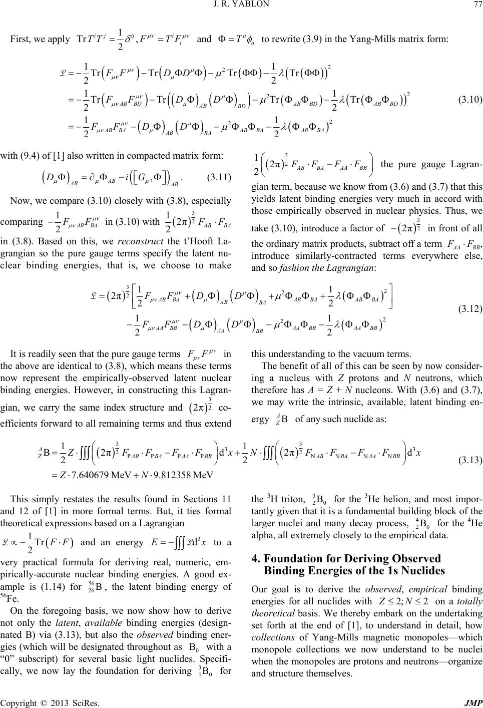

J. R. YABLON 77
First, we apply 1
Tr ,
2
ij iji
i
TFTT F


 
and a
a
T

 to rewrite (3.9) in the Yang-Mills matrix form:
 
 




  



2
2
2
2
2
11
Tr TrTr
22
11
Tr TrTrTr
22
11
22
ABBDAB BDAB BD
AB BD
AB BAABBAABBA
AB BA
FFD D
FFD D
FF DD

 
 
 
 
 



 
  
  
(3.10)
with (9.4) of [1] also written in compacted matrix form:

,G

  

. (3.11)
Now, we compare (3.10) closely with (3.8), especially
2
Tr

  L

3
2
12π
2AB BAAA BB
FF FF




the pure gauge Lagran-
gian term, because we know from (3.6) and (3.7) that this
yields latent binding energies
those empirically observed in nuclear physics. Thus, we

AB
Di


AB AB
comparing 1
AB BA
2
F
F




in (3.10) with

3
2
12πAB B
2
F
F

A
in
the pure gay the latent nu
ng energies, that ake
(3.8). Based on this, we reconstruct the t’Hooft La-
grangian souge terms specif-
clear bindiis, we choose to m
very much in accord with
take (3.10), introduce a factor of

3
2
2π in front of all
the ordinary matrix products, subtract off a term AABB
F
F

,
introduce similarly-contracted teywhere else,
and so fashion the Lagrangian:
rms ever

 




2
2
11
22
AA BBAA BBAA BB
AA BB
FF D D

 
 



(3.12)
It is readily seenure gauge terms
3
21
2π
2
AB BAAB
FF DD

 




L2
21
2
AB BAABBA
BA





F
F that the p


in
the above are identical to (3.8), which means these terms
ow represent the empiricallytent nuclear
biis Lag
this understanding to the vacuum terms.
The benefit of all of this can be seen by now consider-
ing a nucleus with Z protons and N neutrons, which
(3.6) and (3.7),
w
n-observed la
nding energies. However, in constructing thran-
gian, we carry the same index structure and

3
2
2π co-
efficients forward to all remaining terms and thus extend
therefore has A = Z + N nucleons. With
e may write the intrinsic, available, latent binding en-
ergy B
A
Z of any such nuclide as:
 
33
33
2d
2
7.640679 MeV9.812358 MeV
BB
2
PP PP
B2πd
2
ZA BBAAABB
2
NN NN
πABBAAA
11
A
Z
FF FFx 


 NF FFF    x
ZN
 
 
 
 
(3.13)
This simply restates th in Sections 11
and 12 of [1] in more formt ties formal
eoretical expressions based on a Lagrangian

e results found
al terms. But, i
th

1Tr
2
F
F L and an energy 3 dEx
L to a
very practical formula for deriving real, numeric, em-
pirically-accurate ergies. A goo
ample is (1.14) for B, the latent binding energy of
B) via (3.13), but also the observed binding ener-
gi
the 3H triton, 3
20
B for the
3He helion, an
tantly given that it is a fundamental building block of the
larger nuclei and many decay process, 4B for the
4He
ta.
rtaking
tail, how
which
monopnuclei
nuclear binding end ex-
56
26
56Fe.
On the foregoing basis, we now show how to derive
not only the latent, available binding energies (design-
nated
es (which will be designated throughout as 0
B with a
“0” subscript) for several basic light nuclides. Specifi-
cally, we now lay the foundation for deriving 3
10
B for
20
alpha, all extremely closely to the empirical da
4. Foundation for Deriving Observed
Binding Energies of the 1s Nuclides
Our goal is to derive the observed, empirical binding
energies for all nuclides with 2; 2ZN on a totally
theoretical basis. We thereby embark on the unde
d most impor-
set forth at the end of [1], to understand in de
collections of Yang-Mills magnetic monopoles—
ole collections we now understand to be
when the monopoles are protons and neutrons—organize
and structure themselves.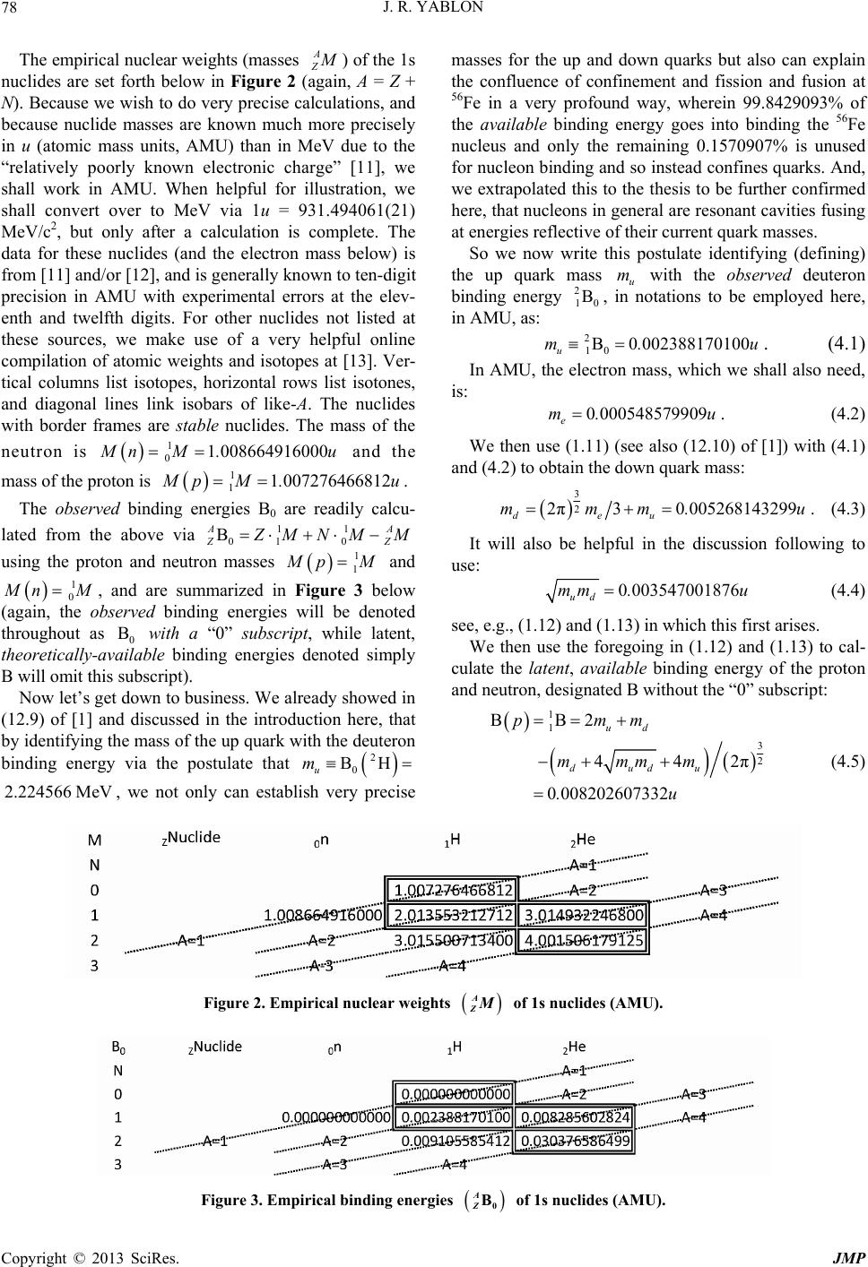

J. R. YABLON 78
The empirical nuclear weights (masses A
Z
M
) of the 1s
nuclides are set forth below in Figure 2 (again, A = Z +
N). Because we wish to do very precise calculations, and
because nuclide masses are known much more precisely
in u (atomic mass units, AMU) than in MeV due to the
“relatively poorly known electronic charge” [11], we
shall work in AMU. When helpful for illustration, we
shall convert over to MeV via 1u = 931.494061(21)
MeV/c2, but only after a calculation is complete. The
data for these nuclides (and the electron mass below) is
from [11] and/or [12], and is generally known to ten-digit
precision in AMU with experimental errors at the elev-
enth and twelfth digits. For other nuclides not listed at
these sources, we make use of a very helpful online
compilation of atomic weights and isotopes at [13]. Ver-
tical columns list isotopes, horizontal rows list isotones,
and diagonal lines link isobars of like-A. The nuclides
with border frames are stable nuclides. The mass of the
neutron is

1
01 008664916000
M
nM. u and the
mass of the proton is

1
11007276466812
M
pM. u .
The observed binding energies B0 are readily calcu-
lated from the above via 11
01 0
B
AA
ZZ
Z
MNM M 
using the proton and neutron masses

1
1
M
pM and

1
0
M
nM, ae 3 below nd are summarized in Figur
nding energies will be denoted
energies denoted simply
already show
(12.9) of [1]
(again, the observed bi
throughout as 0 B with a “0” subscript, while latent,
theoretically-available binding
B will omit this subscript).
Now let’s get down to business. We ed in
and discussed in the introduction here, that
by identifying the mass of the up quark with the deuteron
binding energy via the postulate that


2
0
BH
u
m
2.224566 MeV , we not only can establish very precise
masses for the up and down quarks but also can explain
the confluence of confinement and fission and fusion at
56Fe in a very profound way, wherein 99.8429093% of
the available binding energy goes into binding the 56Fe
nucleus and only the remaining 0.1570907% is unused
for nucleon binding and so instead confines quarks. And,
we extrapolated this to the thesis to be further confirmed
here, that nucleons in general are resonant cavities fusing
at energies reflective of their current quark masses.
So we now write this postulate identifying (defining)
the up quark mass u with the observed deuteron
binding energy , in notations to be employed here,
in AMU, as:
m
2
10
B
2
10
B0 002388170100
u
m. u
0 000548579909
e
m. u
. (4.1)
In AMU, the electron mass, which we shall also need,
is:
. (4.2)

We then use (1.11) (see also (12.10) of [1]) with (4.1)
and (4.2) to obtain the down quark mass:

3
2
2π30 005268143299
deu
mmm.u . (4.3)
It will also be helpful in the discussion following to
use:
0 003547001876
ud
mm .u (4.4)
see, e.g., (1.12) and (1.13) in which this first arises.
We then use the foregoing in (1.12) and (1.13) to cal-
culate the latent, available binding energy of the proton
and neutron, designated B without the “0” subscript:




1
1
3
2
BB2
442π
0 008202607332
ud
dudu
pmm
mmmm
.u
 
 

(4.5)
Figure 2. Empirical nuclear weights


A
ZM of 1s nuclides (AMU).
Figure 3. Empirical binding energies


A
Z0
B of 1s nuclides (AMU).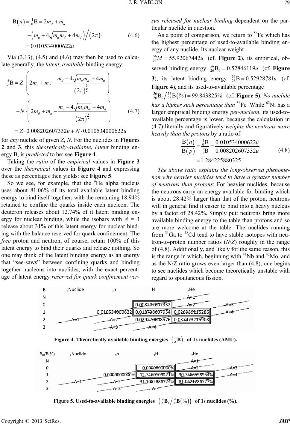

J. R. YABLON 79



1
0
BB2
44
0 010534000622
du
uu
nm
mmm
.u
 


3
2
2π
dd
m
m (4.6)
Via (3.13), (4.5) and (4.6) may then be used to calcu-
late generally, the latent, available binding energy:


3
2
44
B2
2π
44
2
0 0082026073320010534000622
dudu A
Zud
uudd
mmmm
Zmm
mmmm
Nmm 3
2
2π
du
Z
.uN.u










 
 
(4.7)
for any nuclide of given Z, N. For the nuclides in Figures
2 and 3, this theoretically-available, latent binding en-
ergy B, is predicted to be: see Figure 4.
Taking the ratio of the empirica l values in Figure 3
over the theoretical values in Figure 4 and expre
these as percentages then yields: see Figure 5.
So we see, for example, that the 4He alpha nucleus
uses about 81.06% of its total available latent binding
sus released for nuclear binding dependent on the par-
ticular nuclide in question.
As a point of comparison, we return to 56Fe which has
the highest percentage of used-to-available binding en-
ergy of any nuclide. Its nuclear weight
56
26 55 92067442
M

.u (cf. Figure 2), its empirical, ob-
rved 0 52846119.u (cf. Figure
ailable percentage



ssing
energy to bind itself together, with the remaining 18.94%
retained to confine the quarks inside each nucleon. The
deuteron releases about 12.74% of it latent binding en-
ergy for nuclear binding, while the isobars with A = 3
release about 31% of this latent energy for nuclear bind-
ing with the balance reserved for quark confinement. The
free proton and neutron, of course, retain 100% of this
latent energy to bind their quarks and release nothing. So
one may think of the latent binding energy as an energy
that “see-saws” between confining quarks and binding
together nucleons into nuclides, with the exact percent-
age of latent energy reserved for quark confinement ver-
se binding energy 56
26 0
B
3), its latent binding energy 56
26 B0 52928781.u (cf.
Figure 4), and its used-to-av


56
eon, its used-to-
available percentage
tively weights the n
56
26026
BB99843825%. % (cf. Figure 5). No nuclide
has a higher such percentage than 56Fe. While 62Ni has a
larger empirical binding energy per-nucl
is lower, because the calculation in
(4.7) literally and figuraeutrons more
heavily than the protons by a ratio of:



1
0
1
BB0 010534000622
B0 008202607332B
n.u
p. u

1
2% lare proton, neutrons
will in general find it easier to bind into a he
by a factor of 28.42%. Simply put: neutrons
available binding energy to the table than protons and so
ar
1284225880325.
The above ratio explains the long-observed phenome-
non why heavier nuclides tend to have a greater number
of neutrons than protons: For heavier nuclides, because
the neutrons carry an energy available for binding which
is about 28.4ger than that of th
(4.8)
avy nucleus
bring more
e more welcome at the table. The nuclides running
from 31Ga to 48Cd tend to have stable isotopes with neu-
tron-to-proton number ratios (N/Z) roughly in the range
of (4.8). Additionally, and likely for the same reason, this
is the range in which, beginning with 41Nb and 42Mo, and
as the N/Z ratio grows even larger than (4.8), one begins
to see nuclides which become theoretically unstable with
regard to spontaneous fission.
nergies Figure 4. Theoretically available binding


A
ZB of 1s nuclides (AM eU).




%
AA
ZZ0
BB of 1s nuclides (%). Figure 5. Used-to-available binding energies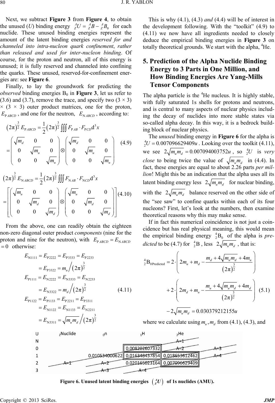

J. R. YABLON 80
Next, we subtract Figure 3 from Figure 4, to obtain
the unused (U) b0
AAA
ZZZ
UBB for each
nuclide. Thesnergies represent the
amount of the latent binding energies reserved for and
channeled into intra-nucleon quark confinement, rather
than released and used for inter-nucleon binding. Of
course, for the proton and neutron, all of this energy is
unused; it is fully re
e quarks. These unu
gi
inding energy
e unused binding e
served and channeled into confining
sed, reserved-for-confinement ener- th
es are: see Figure 6.
Finally, to lay the groundwork for predicting the
observed binding energies B0 in Figure 3, let us refer to
(3.6) and (3.7), remove the trace, and specify two (3 × 3)
× (3 × 3) outer product matrices, one for the proton,
PABCD
E, and one for the neutron, NABCD E, according to:
 
33
3
22
PPP
1
2π2πd
2
00
ABCDAB CD
EFFx
m



00
0000
0000
dd
uu
uu
m
mm
mm
 
 



(4.9)
 
 
33
22
NN
3
N
2π2πd
2
00 00
0000
00 00
ABCDABCD
uu
dd
dd
EFFx
mm
mm
mm





  
 





(4.10)
From the above, one can readily obtain the eighteen
non-zero diagonal outer product components (nine for the
proton and nine for thPNABCDABCD EE
1

e neutron), with

0 otherwise:



N1111P2222 P
P3322
P1111 N2222N
3333 P2233
3
2
N1122 N1133 N2211
3
2
N3311
2π
2π
u
ud
EEEE
Em
EEE E
EEE
Emm





This is why (4.1), (4.3) and (4.4) will be of interest in
the development following. With the “toolkit” (4.9) to
(4.11) we now have all ingredients needed to closely
deduce the empirical binding energies in Figure 3 on
totally theoretical grounds. We start with the alpha, 4He.
5. Prediction of the Alpha Nuclide Binding
Energy to 3 Parts in One Million, and
ia
d-
ing
a is
4
2Uing over the toolkit (4.11),
3333 N2233
3
2
N3322
P1122P1133 P2211 P3311
2π
d
Em
EEEE



(4.11)

How Binding Energies Are Yang-Mills
Tensor Components
The alpha particle is the 4He nucleus. It is highly stable,
with fully saturated 1s shells for protons and neutrons,
and is central to many aspects of nuclear physics includ-
ing the decay of nuclides into more stable states v
so-called alpha decay. In this way, it is a bedrock buil
block of nuclear physics.
The unused binding energy in Figure 6 for the alph
0 007096629409.u. Look
we see 20 007094003752
ud
mm .u, so 4
2U is very
close to being twice the value of
ud
mm in (4.4). In
fact, these energies are equal to about 2.26 parts per mil-
lion! Might this be an indication that the alpha uses all its
latent binding energy less 2ud mm for nuclear binding,
wi th the 2ud mm balance reserved on the other side of
e quarks within each of its four the “see saw” to confin
First, let’s look at the numben
ke sense
less
nucleons? ers, th examine
theoretical reasons why this may ma.
If in fact this numerical coincidence is not just a coin-
cidence but has real physical meaning, this would mean
the empirical binding energy 4
20
B of the alpha is pre-
dicted to be (4.7) for 4
2B, 2m ud
m, that is:


4
2 0Predicted3
2
44
B22
2π
dudu
ud
mmmm
mm

3
2
44
22
2π
uu dd
du
mm mm
mm


 









(5.1)

20.030379212155
ud
mm u
where we calculate using,
ud
mmfrom (4.1), (4.3), and
Figure 6. Unused latent binding energies


A
ZU of 1s nuclides (AMU).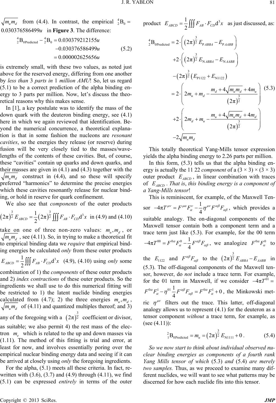

J. R. YABLON 81
ud
mm from (4.4). In contrast,irical 4
20
B the emp

0.030376586499u in Figure 3. The difference:
0379212155
0376586499
0002625656
u
u
u
(5.2)
is extremely small, with these two values, as noted just
above for the reserved energy, differing from one another
less than 3 parts in 1
.1) to ng en-
ergy to theo
retical reasons why
In [1], a key postulate was to identify the mass of the
down quark with the deuteron binding ener
here in which we again reviewed that iden
yond the numerical concurrence, a theoretical explana-
44
2 0Predicted2 0
BB 0.03
0.03
0.00



by million AMU! So, let us regard
(5be a correct prediction of the alpha bindi
3 parts per million. Now, let’s discuss the-
this makes sense.
gy, see (4.1)
tification. Be-
tion is that in some fashion the nucleons are resonant
cavities, so the energies they release (or reserve) during
fusion will be very closely tied to the masses/wave-
lengths of the contents of these cavities. But, of course,
these “cavities” contain up quarks and down quarks, and
their masses are given in (4.1) and (4.3) together with the
ud
mm construct in (4.4), and so these will specify
preferred “harmonics” to determine the precise energies
which these cavities resonantly release for nuclear bind-
ing, or hold in reserve for quark confinement.
We also see that components of the outer products
 
33
3
22
1
2π2πd
2
ABCDAB CD
EFFx
 in (4.9) and (4.10)
take on one of three non-zero values: ,
ud
mm, or
ud
mm , see (4.11). So, in trying to make a theoretical fit
to empirical binding data we require that empirical bind-
ing energies be calculated only from these outer products
3
1d
2
ABCDABCD
EFFx
 (4.9), (4.10) using only some
combination of 1) the components of these outer products
d 2) index contractions of these outer products. So the an
ingredients we shall use to do this nu
be restricted to 1) the latent nuclide binding energies
s u
m
merical fitting will
calculated from (4.7); 2) the three energie,d
m,
ud
mm of (4.11) and quantized multiples thereof; and 3)
any of the foregoing with a

3
2
2π coefficient or divisor,
as suitable; we also permit 4) the rest mass of the elec-
to the up and down masses via tron e
m which is related
act, re
itten
(5.1) ca
product 3
1d
2
ABCDABCD
EFFx
 as just discussed, as:


 
(1.11). The method of this fitting is trial and error, at
least for now, and involves essentially poring over the
empirical nuclear binding energy data and seeing if it can
be arrived at closely using only the foregoing ingredients.
For the alpha, (5.1) meets all these criteria. In f-
wr with (3.6), (3.7) and (4.9) through (4.11), we find
n be expressed entirely in terms of the outer


3
42
2 0PredictedPP
3
2NN
3
21122
B22π
22π
2π
44
ABBA AABB
ABBA AABB
d
EE
EE
EE
mmmm

 



 




(5.3)
.
tually the 11 22 componen
outer product ABCD
E, in linear combination with traces
of ABCD E. That is, this binding energy is a component of
a Yang-Mills tensor!
This is reminiscent, for example, of the Maxwell Ten-
sor
P1122 N

3
22 u
du
ud
mm

  

2
3
2
2π
44
22
2π
2
uu dd
du
ud
mm mm
mm
mm





 




This totally theoretical Yang-Mills tensor expression
yields the alpha binding energy to 2.26 parts per million.
In this form, (53) tells us that the alpha binding en-
ergy is act of a (3 × 3) × (3 × 3)
1
4π
4
TFF FF
 


  , which provides a
suitable analogy. The on-diagonal components of the
Maxwell tensor contain both a component term and a
trace term just like (5.3). For example, for the 00 term
00001
4π
4
TFF FF



 , we analogize 00 F

F

to
the 1122 E and
F
F



to the

3
2
2πABBA AABB EE in
(5.3). The off-diagonal components of the Maxwell ten-
sor, however, do not include a trace term. For example,
for the 01 term in Maxwell, if we consider 01
4πT

01 0101
1
FF

0
4FF FF
 


, the Minkowski met-
ric



filters out the trace. This latter, off-diagonal
an

alogy allows us to represent (4.1) for the deuteron as a
tensor component without a trace term, for example, as
(see (4.11)):
3
2
1 0Predicted
B2N1111 2π0
u
mE

. (5.4)
r binding energies as compone
So we now start to think about individual observed nu-
clea nts of a fourth rank
Yang Mills tensor of which (5.3) and (5.4) are merely
two samples. Thus, as we proceed to examine many dif-
ferent nuclides, we will want to see what patterns may be
discerned for how each nuclide fits into this tensor.

J. R. YABLON 82
Physically, the alpha partiotons
two neutrons, in terms of qnd
quarks enter (5.3) in
letemetric relative to the do
cle contains two prand
uarks, six up quarks a six
down quarks. It is seen that the upa
comply symfashion wn
quarks, i.e., that (5.3) is invariant under the interchange
ud
mm. The factor of 2 in front of ud mm of course
means that two components of the outer produc t are also
involved. So we have preliminarily associated 2ud mm

n pair and the proton
P1122
EE so that t
ea
N1122
ch c
he neutro
pairontribute 1ud mm to (5.3), and (5.3) thereby
remains absolutely symmetric not only under ud

,
but also under pn interchange.
We do note that there is some flexibility in these as-
signments of energy numbers to tensor components, be-
ud
, cause each of ,mm ud mm in the (4
ral different components of the outer
l nu-
cl
is such a ng energ
per million. C
atter deu
d the
mwoto bind the proton
473215908 , an
.11) toolkit is
associated
pr
with seve
oduct. So the choice of 1122 E in (5.3) (while requiring
pn symmetry) and of N111 1 E in (5.4) is flexible
versus the other available possibilities in (4.11), and
should be revisited once we study other nuclides not yet
considered and seek to understand the more general
Yang-Mills tensor structure of which the individua
ide binding energies are components.
One other physical observation is also very noteworthy,
and to facilitate this discussion we include the well-
known “per-nucleon” binding graph as Figure 1 above.
One perplexing mystery of nuclear physics is why there
large “chasm” between bindiies for the
2H, 3H and 3He nuclides, and the biding energy of the
4He nuclide which we have now predicted to within parts
ontrasting (5.3) for 4He with (5.4) for 2H,
we see that for the lteron, we “start at the bot-
tom” with 1
10
B0 for 1H (the free proton), ann
“add” 2B0rth of energy
10 u
d the neutron together into 2H. Conversely, for the al-
pha we “start at the top” with the total latent binding en-
ergy 4
2B0 037.ud then subtract off
an
2ud mm , to match the empirical data with
4037473215908 2.um. But as we learned
in Section 12 of [1] and have reiterated here, any time we
do not use some of the latent energy for nuclear binding,
that unused energy remains behind in reserve to confine
the quarks in a type of nuclear see-saw.
So what we learn is that for the alpha particle, a total
of
20
B 0ud m
20 007094004
ud
mm .uis held in reserve to con-
fine the quarks, while the majority balance is released to
bind the nucleons to one another. In contrast, for the
deuteron, a total of 2
10
B0 002388170100
u
m. u is
released for inter-nucleon binding while the majority
balance is held in reserve to confine the quarks.
Now to the point: for some nuclides (e.g. the deuteron)
the question is: how much energy is released from quark
confinement to bind nucleons? This is a “bottom to top”
nuclide. For uclides (e.g., the alpha) the question
is: howgy is reserved out of the theoretical
maximum available, to confine quarks. This is a “top to
bottom” nuclide. For top to bottom nuclides, there is a
scalarls tensors. For bottom to
other n
much ener
trace in the Yang-Mil top
nuclides or analogy,
one may suppose that somewhere
there is not. Using the Maxwell tens
there is a Kronecker
delta A
B

and/or AB
CD

which filters out the trace from
“off-diagonal” terms and leaves the trace intact for “on-
diagonal” terms. In this way, the “bottom to top” nu-
clides are “off-diagonal” tensor components and the “top
to bottom” nuclides are “on diagonal” components. In
either case, however, the “resonance” for nuclear binding
is established by the components of the NABCD E, which
are ,
ud
mm, ud mm in some combination and/or inte-
ger multiple. And, as regards Figure 1 above, the chasm
between the lighter nuclides and 4He is explained on the
basis that each of 2H, 3H and 3He are “bottom to top”
“o 4 ff-diagonal” nuclides, while He, which happens to fill
the 1s shells, is the lightest “top to bottom” “on-diago-
nal” nuclide. 2H, 3H and 3He start at the bottom of the
nuclear see-saw and move up; 4He starts at the top of the
see-saw and moves down.
To amplify this point, in Figure 7 below we peek
ahead at some heavier nuclides, namely, 3Li and 4Be.
Using a nuclear shell model similar to that used for elec-
tron structure, all nucleons in the 4He alpha are in 1s
shells. The two protons are spin up and down each with
1s, as ar the two netrons. As soon as we add one more
nucleon, by Exclusion, we must jump up to the 2s shell,
which admits four more nucleons and can reach up to
8
4Be before we must make an incursion into the 2p shell.
We note immediately from the above—which has been
noticed by others before—that the binding energy
8
40
B0 060654752.u of
8Be is almost twice as large as
that of the alpha particle, to just under one part in ten
thousand AMU. Specifically:
48
20 40
2BB20 030376586499
0 060654752
0.000098421
.u
.u
u



(5.5)
This is part of why 8Be is unstable and invariably de-
cays almost immediately into two alpha particles (9Be is
the stable Be isotope). But
e u
of particular interest here, is
to
thre
subtract off the alpha 4
20
B0 030376586499.u from
each of the Li and Be isotopes, and compare them side
by side with the non-zero binding energies from H and
He. The result of this exercise is in Figure 8 below.
Equation (5.5) is represented above by the fact that
84 4
40 202
BB B. The table on the left is a “1s square”
and the table on the right is a “2s square.” But they are
both “s-squares.” What is of interest is that the remaining
e nuclides in the 2s square are not dissimilar in pat-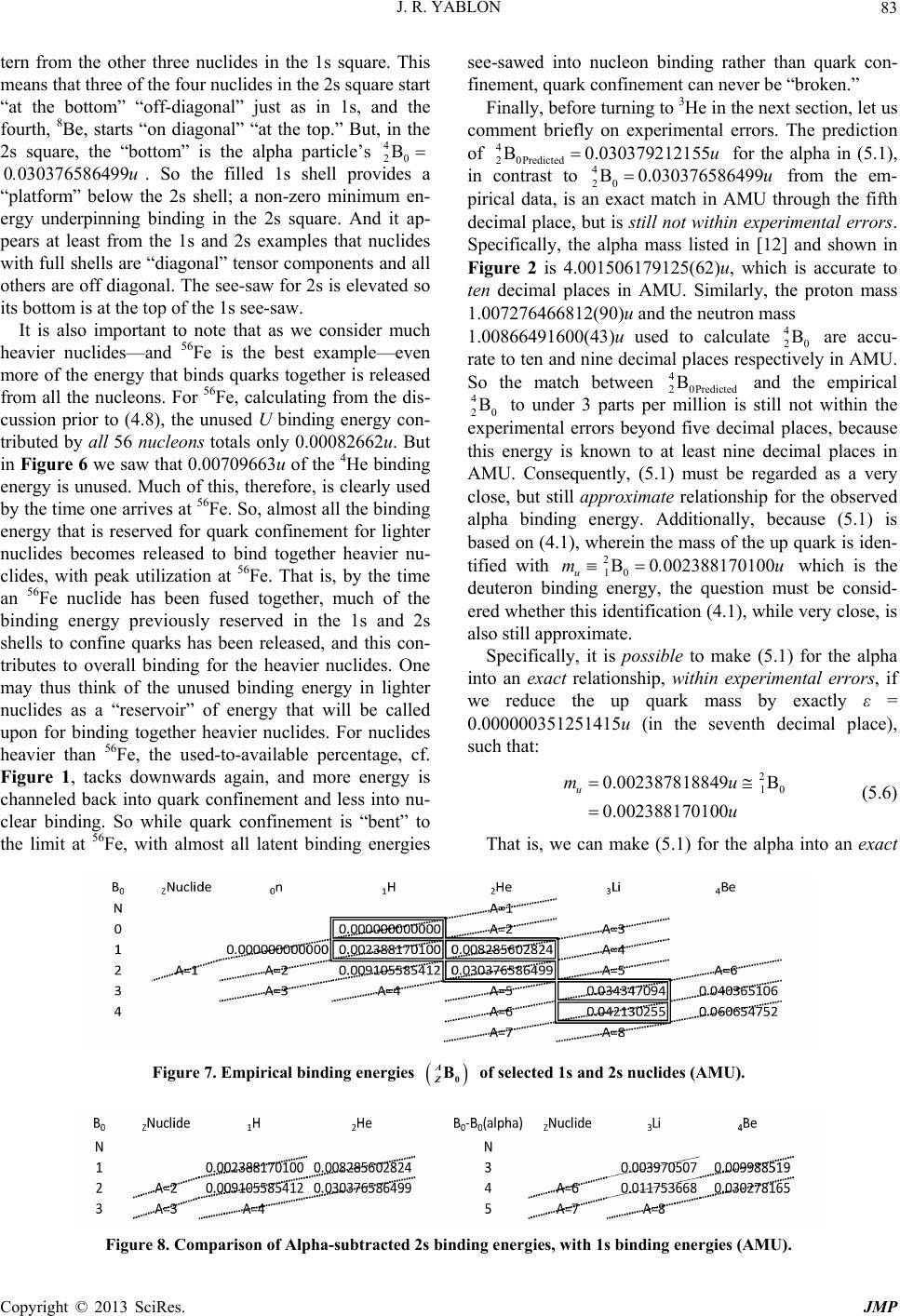

J. R. YABLON
ight ©s. JMP
83
te
“at the bottom” “of
e alpharticle’s 4
20
B
rn from the other three nuclides in the 1s square. This
means that three of the four nuclides in the 2s square start
f-diagonal” just as in 1s, and the
fourth, 8Be, starts “on diagonal” “at the top.” But, in the
2s square, the “bottom” is th pa

0376586499.u. So the filled 1s shell provides a
” below the 2s shell; a non-zeminimum en-
nderpinning binding in the 2e.
least from the 1s and 2s e nuclides
of 4
20Predicted
B 0.030379212155u for the alpha in (5.1),
in contrast to 4
20
B 0.030376586499u from the em-
pirical data, is an exact match in AMU through the fifth
decimal place, but is still not within experimental errors.
Specifically, the alpha mass listed in [12] and shown in
Figure 2 is 4.001506179125(62)u, which is accurate to
ten decimal places in AMU. Similarly, the proton mass
1.00727646681 2(90)u and the neutron mass
1.00866491600 (43)u used to calculate 4
20
B are accu-
rate to ten and nine decimal places respectively in AMU.
So the match between 4
2 0Predicted
B and the empirical
4
20
B to under 3 parts per million is still not within the
experimental errors beyond five decimal places, because
this energy is known to at least nine decimal places in
AMU. Consequently, (5.1) must be regarded as a very
close, but still approximate relationship for the observed
alpha binding energy. Additionally, because (5.1) is
based on (4.1), wherein the mass of the up quark is iden-
tified with 2
10
B0 002388170100
u
m. u which is the
deuteron binding energy, the question must be consid-
ered whether this identification (4.1), while very close, is
also still approximate.
Specifically, it is possible to make (5.1) for the alpha
into an exact relationship, within experimental errors, if
we reduce the up quark mass by exactly ε =
0.00000035125 1415u (in the seventh decimal place),
such that:
2
10
0.002387818849 B
0.0023881701 00
u
mu
u

 (5.6)
That is, we can make (5.1) for the alpha into an exact
0 03
“platform
ergy u
pears at
wi
tribute
ro
s squar
xamples that
And it ap-
th full shells are “diagonal” tensor components and all
others are off diagonal. The see-saw for 2s is elevated so
its bottom is at the top of the 1s see-saw.
It is also important to note that as we consider much
heavier nuclides—and 56Fe is the best example—even
more of the energy that binds quarks together is released
from all the nucleons. For 56Fe, calculating from the dis-
cussion prior to (4.8), the unused U binding energy con-
d by all 56 nucleons totals only 0.00082662u. But
in Figure 6 we saw that 0.00709663u of the 4He binding
energy is unused. Much of this, therefore, is clearly used
by the time one arrives at 56Fe. So, almost all the binding
energy that is reserved for quark confinement for lighter
nuclides becomes released to bind together heavier nu-
clides, with peak utilization at 56Fe. That is, by the time
an 56Fe nuclide has been fused together, much of the
binding energy previously reserved in the 1s and 2s
shells to confine quarks has been released, and this con-
tributes to overall binding for the heavier nuclides. One
may thus think of the unused binding energy in lighter
nuclides as a “reservoir” of energy that will be called
upon for binding together heavier nuclides. For nuclides
heavier than 56Fe, the used-to-available percentage, cf.
Figure 1, tacks downwards again, and more energy is
channeled back into quark confinement and less into nu-
clear binding. So while quark confinement is “bent” to
the limit at 56Fe, with almost all latent binding energies
see-sawed into nucleon binding rather than quark con-
finement, quark confinement can never be “broken.”
Finally, before turning to 3He in the next section, let us
comment briefly on experimental errors. The prediction
Figure 7. Empirical binding energies


0
B of selected 1s and 2s nuclides (AMU).
A
Z
inding energies, with 1s binding energies (AMU). Figure 8. Comparison of Alpha-subtracted 2s b
Copyr 2013 SciRe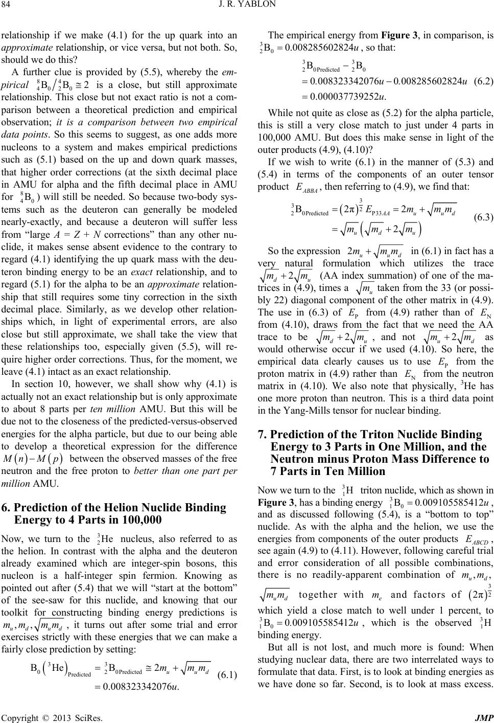

J. R. YABLON 84
relationship if we make (4.1) for the up quark into an
approximate relationship, or vice versa, but not both. So,
should we do this?
A further clue is provided by (5.5), whereby the em-
pirical 84
0
BB2 is a close
but not exact rat
al place
n can ge
near
gard (4.1) identifying the up quark mass with the deu-
teron binding energy to be an exact relationship, and to
regard (5.1) for the alpha to be an approximate relation-
ship that still requires some tiny correction in the sixth
decimal place. Similarly, as we develop other relation-
ships which, in light of experimental errors, are also
close but still approximate, we shall take the view that
these relationships too, especially given (5.5), will re-
quire higher order corrections. Thus, for the moment, we
leave (4.1) intact as
In section 10, however, we shall show why (4.1) is
not an exact relationship but is only approximate
to about 8 parts per ten million AMU. But this will be
due not to the closeness of the predicted-versus-observed
energies for the alpha particle, but due to our being able
to develop a theoretical expression for the difference
 
402, but still approximate
relationship. This close io is not a com-
parison between a theoretical prediction and empirical
observation; it is a comparison between two empirical
data points. So this seems to suggest, as one adds more
nucleons to a system and makes empirical predictions
such as (5.1) based on the up and down quark masses,
that higher order corrections (at the sixth decim
in AMU for alpha and the fifth decimal place in AMU
for 8
40
B) will still be needed. So because two-body sys-
tems such as the deuteronerally be modeled
ly-exactly, and because a deuteron will suffer less
from “large A = Z + N corrections” than any other nu-
clide, it makes sense absent evidence to the contrary to
re
an exact relationship.
actually
M
nMp between the observed masses of the free
utron and tnehe free proton to better than one part per
million AMU.
6. Prediction of the Helion Nuclide Binding
Energy to 4 Parts in 100,000
Now, we turn to the 3
2He nucleus, also referred to as
the helion. In contrast with the alpha and the deuteron
already examined which are integer-spin bosons, this
nucleon is a half-integer spin fermion. Knowing as
pointed out after (5.4) that we will “start at the bottom”
of the see-saw for this nuclide, and knowing that our
toolkit for constructing binding energy predictions is
,,
ud ud
mm mm, it turns out after some trial and error
exercises strictly with these energies that we can make a
fairlose prediction by setting:

The empirical energy from Figure 3, in comparison, is
3
20
B 0.008285602824u, so that:
33
2 0Predicted2 0
BB
602824
0.000037739252 .u



(6.2)
While not quite as close as (5.2) for the alpha particle,
this is still a very clos
00083233420760 008285.u.u
tch to just under 4 parts in
10
n
ABBA , then referring to (4.9), we find that:

e ma
0,000 AMU. But does this make sense in light of the
outer products (4.9), (4.10)?
If we wish to write (6.1) in the manner of (5.3) ad
(5.4) in terms of the components of an outer tensor
product E

3
32
2 0PredictedP33
B2π2
2
AA u
Em
mm m


So the expression
u d
mm
(6.3)
ud u
2uud mmm in (6.1) in fact has a
very natural formulation which utilizes the trace
2
du
mm (AA index summation) of one of the ma-
trices in (4.9), times a u mtaken from the 33 (or possi-
bly 22) diagonal component of the other matrix in (4.9).
The use in (6.3) of P E from (4.9) rather than of N E
from (4.10), draws from the fact that we need the AA
trace to be 2
du
mm, and not 2
ud
mm as
would otherwise occur if we used (4.10). Shere, the
empirical data clearly causes us to use P Eom the
from the neutron
matrix in (4.10). We also note that physically, 3He has
one more proton than neutron. This is a third data point
in the Yang-Mills tensor for nuclear binding.
7. Prediction of the Triton Nuclide Binding
Energy to 3 Parts in One Million, and the
Neutron minus Proton Mass Difference to
o
fr
proton matrix in (4.9) rather than N
E
7 Parts in Ten Million
Now we turn to the 3
1H triton nuclide, which as shown in
Figure 3, has a binding energy 3
10
B0 009105585412.u,
and as discussed following (5.4), is a “bottom to top”
nuclide. As with the alpha and the helion, we use the
energies from components of the outer products ABCD E,
see again (4.9) to (4.11). However, following careful trial
and error consideration of all possible combinations,
there is no readily-apparent combination of ,,
ud
mm
ud
mm together with e m and factors of

3
2
2π
which yield a close match to well under
3
1 percent, to
B
10 0 009105585412.u, which is the observed 3 1H
binding energy.
But all is not lost, and much more is found: When
studying nuclear data, there are two interrelated ways to
formulate that data. First, is to look at binding energies as
we have done so far. Second, is to look at mass excess.
y cl
33
02 0Predicted
Predicted
BHeB 2
0.008323342076 .
uud
mmm
u


(6.1)

J. R. YABLON 85
The latter form
ach that enables us to match
up the empirical binding data for the triton to the
ulation, mass excess, is very helpful when
studying nuclear fusion and fission processes, and as we
shall now see, it is this appro
,, ,
dud e
mmmmm and factors of

u
3
2
2π that we have
ployedalready successfully em for the deuteron, alpha,
and helion. As a tremendous bonus, we will be able to
derive a strictly theoretical expression for the observed,
empirical difference:
 
11
010.001388449 188
M
nMpM Mu (7.1)
between the free, unbound neutron mass


M
n

1 008664916000.u and the free, unbound proton mass

1 007276466812
M
p. u, see Figure 2.
The derivation of the 3He binding energy and the neu-
tron minus proton mass difference is somewhat involved,
and so is detailed in the Appendix. But the results a
follows: For the neutron minus proton mass differen
(A15), also using (1.11), we obtain:
re as
ce, in
 
Predicted
 



3
2
3
2
22π
3232π
ue μd
ud μdu
MnM p
mm mm
mm mmm


 
g energy in (A17), we use
th
0.001389166099u
which differs from the empirical (7.1) by a mere
0.000000716911u, or just over seven parts per ten mil-
lion! And for the 3He bindin
(7.2)
e above to help obtain:


33
10Predicted
Predicted
BH B
0
3
2
42 2π
0.009102256308
uμd
mmm
u


(7.3)
whic 9105585412u, the em-
pi
A theoretic
uct
h differs from 3
10
B 0.00
e 3, by merrical value in Figur 0.000003329104u,
or just over 3 parts per million.
al tensor expression for (7.3) using compo-
nents of an outer prodABBA E as in (5.3), (5.4) and
(6.3), may be written as:

ely


3
32
1 0PredictedP2233P3322
P1122P1133
3
2
2π
42 2π
uμd
BEEEE
EE
mmm
 


(7.4)
As earlier noted following (5.4), there will be some
flexibility in these tensor component assignments until
we develop a wider swathe of binding energ
P2222 P3333
ies beyond
f
de
bin
mi e have also deduced a
e n
g
l
ct theo
nding
energies
8. Mass Excess Pred
the “1s square” and start to discern the wider patterns.
With the foregoing, we have now reached our goal o
ducing precise theoretical expressions for all of the 1s
ding energies, solely as a function of elementary fer-
on masses. In the process, w
like-expression for theutron-proton mass difference!
From here, after consolidatin our binding energy re-
sults and expressing them as mass excess in Section 8,
we examine the solar fusion cycle in Section 9, including
possible technological implications of these resuts for
catalyzing nuclear fusion. In Section 10 we again focus
on experimental errors as we did at the end of Section 5,
and explain why (7.2) should be taken as an exa -
retical relationship with the quark masses and bi
then slightly recalibrated.
ictions
Let us now aggregate some of the results so far, as well
as those in the Appendix. First of all, let us draw on (A4),
and use (A14) and the neutron minus proton mass dif-
ference (7.2) to rewrite (A4) as:



3
1 Predicted
3
2
2
42 2π
uμd
MMpMn
mmm

 (8.1)
Specifically, we have refashioned (A4) to include one
proton mass and two neutron masses, because the 3
1H
triton nuclide in fact contains one proton and two neu-
trons. Thus,

3
2
42 2π
uμd
mmm represents a theo-
retical value of the mass excess of two free neutrons and
one free proton with


2
M
pMn over the mass
they possess when fused into a triton, expressed
equal in
Similarly for heliu
via a
negative number as a fusion mass loss. This is
magnitude and opposite in sign to binding energy (7.3).
m nuclei, first we use (A5) to write:
 
3113
201 0 2
3
2
B2
2
MMM
M
pMnM
 

(8.2)
We then place 3
2
M
on the left and use (6.1) to write:




3
222 uud
M
Mp Mnmmm. (8.3)
Here, 2uud mmm is the fusion mass loss for the
helion, also equal and opposite to binding energy (6.1).
Next, we again use (A5) to write:
 
4114
2010 2
4
2
B22
22
MMM
M
pMnM
 
 (8.4)
Combining this with (5.1) then yields:





4
22266
10 10
ud
du
MMpMnmm
mm


3
2
16 2
2π
ud
ud
mm mm
(8.5)

J. R. YABLON
Copyright © 20 JMP
86
The fusion mass loss for the alpha—much larger than
for the other nuclides we have examined—is given by the
lengthie
 
22
13 SciRes.
r terms after
M
pMn. Agai
equaha binding energy
with terms consolidated above.
via (A5), it is easy to
n, this is
in (5.1), l and opposite to the alp
Finally, from (4.1),deduce for
the deuteron, that:



2
1u
M
Mp Mnm, (8.6)
etical Review of the
pr
mine that an energy (A11) is released in this fusion,
which energy, in light of (A13), now becom

9. A Theor Solar Fusion
Cycle, and a Possible Approach to
Catalyzing Fusion Energy Release
As a practical exercise, let us now use all of the forego-
ing results to theoretically examine the solar fusion cycle.
The first step in this cycle is (A10) for the fusion of two
otons into a deuteron. It is from (A10) that we deter-
with a mass loss represented simply by u m, again,
equal and opposite the bindingy (4.1).
es:
energ

3
2
2π0 01141003
d
m.u (9.1)
11 2
11 1
Energy HHHEnergy20045
μ
em 

 
This equates to 0.420235 MeV which is a well-k
energy in solar fusion as is noted in the Appendix. The
positron annihilates with an electron ee
nown



 to
pr
where in deuterons produced in (9.1) fuse with pr
prelions. We wri
2
otons to
oduce hte this in terms of masses as:
321
11
Energy
M
M
1
M. (9.3)
The proton mass is 1
oduce an additional e
m2 worth of energy as well.
The second reaction in the solar fusion cycle is:
21 3
11 2
HH HeEnergy  (9.2)
M
, and these other two masses
have already been found, respectively, i
Thus, (9.3) may be reduced to:
n (8.6) and (8.3).


21 3
11 2
EnergyHHHe Energy 
which equates to 5.528577 MeV, also a well-known en-
ergy in the study of solar fusion.
The final step in this cycle fuses two helions together
0 005935171976
ud
mm. u
u
m (9.4)
to
of this relationship is as follows:
33411
22211
Energy
The mass equivalent
M
MMMM (9.6)
yield alpha particles plus protons, which protons then
are available to repeat the cycle starting at (9.1):
33 411
22 211
HeHeHeHH Energy (9.5)
Here we again make use of

1
1
M
Mp, together with
(8.3) and (8.5) to write:



3
2
41010 162π
dudd u
mmm mmm 
33 411
22 211
EnergyHeHeHeHHEnergy2
0 0137
u
m
.
 

This equates to 12.791768 Me
6
3252
ud
m (9.7)
V, which is also a
well-known energy from solar fusion studies.
g. [14]), the reaction
he two 3He which
8003u
Now, as is well known (see, e.
(9.4) must occur twice to produce t2
are input to (9.7), and the reaction (9.1) must occur twice
to produce the two 2
1H which are in turn input to (9.4).
So pulling this all together from (9.1), (9.4), (9.7) and
ee



, we may express the entire solar fusion
. In the top line b
detail each energy release from large
ions
each
contribution shown in the top line, including the neutrino
-
sol inate
the
cycle in (9.8) belowelow, we show in
st to smallest, fol-
lowed by the electron and neutrino emiss. In the
second line we segregate in separate parenthesis,
mass which is virtually zero. In the third line, we con
idate terms. In the final line we use (1.11) to elim
electron rest mass:









14
12
Energy4H2He12.79 M2



 

3
2
264
2π
1010 12
du ud
ud ud
du u
mm mm
mmm
3
2
MeV 20.42MeV 42
2224 2
2π
μd
u ude
d
mm
m mmmm
3
2
10 10 16
4642
2π
222
ude ud
ee
mm mm
m
mmm mm
m
eV2 5.5 

   
462 d
ud ud
mm mm

  







 




 


 




 

3
2
733389 MeV
2π
uud
.
12 26 mmm
(9.8)

J. R. YABLON 87
The above shows at least two things. First, the total
energy of approximately 26.73 MeV
leased during solar fusion is expresse
ed!
This portends the ability to do the same for other types of
fusion and fission, once the analysis of this paper is ex-
nded to larger nuclides Z > 2, N > 2.
ons as resonant cavities
w
more
practical, because (9.8) tells us the precise
that go into releasing the total 26.73 MeV of energy in
the above. In particular, if one wanted to create an artifi-
cial “sun in a box,” one would be inclined to amass a
store of hydrogen, and subject that hydrogen store to
g
h
In the above, we have explicitly sho
fre ap
h.
So, what do we learn? If the nucleons are regarded as
resonant cavities and the ener
pend on the masses of their current quarks as is made
ve
and harmonics highlighted in (9.9) and (9.10
for harmonic fusion is to subject a hydroge
high-fre proximate
of with the v
ill catalyze fusion by perhaps
reducing the amount of heat that is required. In pre-
sent-day approaches, fusion reactions are trigge
heat generated from a fission reaction, and
would be to reduce or eliminate this need for such high
as, but not limited to, Compton
backscattering and any other methods which are known
at present or may become known in the future for pro-
ducing gamma radiation, it would also be necessary to
provide substantial shielding against the health effects of
such radiation. The highest energy/smallest wavelength
component, 629 44MeV6 69F
d
m. .
known to be re-
d entirely in terms
of a theoretical combination of the up and down (and
optionally electron) masses, with nothing else add
te
Secondly, because the results throughout this paper
seem to validate modeling nucle
ith energies released or retained based on the masses of
their quark contents, this tells us how to catalyze “reso-
nant fusion” which may make fusion technology
resonances
amma radiation at or near the specified discrete ener-
gies that appear in (9.8), so as to facilitate resonant cav-
ity vibrations at or near the energies required for fusion
to occur. Specifically, one would bathe theydrogen
store with gamma radiation at one or more of the follow-
ing energies/frequencies in combination, some without,
and some with, the Gaussian

3
2
2π divisor (we con-
ths via vert to waveleng


1F1197 MeV):




harmonic13 22 MeV14 91F
ud
mm . .

62944MeV669F
2 22MeV8856F
2harmonic4 45MeV44 28F
4harmonic8 90MeV22 14F
330MeV 5962F
2harmonic6 61MeV29 81F
d
u
u
u
ud
ud
m. .
m. .
m..
m..
mm ..
mm. .






(9.9)
4







3
2
3
2
3
2
3
2
22π0.62 MeV316.15F
10 2π312MeV 6323F
10 2π141MeV139.47F
22 2π3.10 MeV63.40F
d
d
u
u
m
m. .
m.
m




3
2
3
2
3
2
3
2
22π0.42 MeV469 53F
42πharmonic0.84 MeV234.77F
12 2πharmonic2.52 MeV78 26F
16 2πharmon
ud
ud
ud
ud
mm .
mm
mm .
mm




ic3.36 MeV58.69F
(9.10)
wn each basic
quency/energy whichpears in the second, third or
fourth lines of (9.8) as well as harmonics that appear in
(9.8). Also, one should consider frequencies based on the
electron mass and its wavelengt
gies at which they fuse de-
ry evident by (9.8), and given the particular energies
), the idea
n store to
quency gamma radiation at least one
the frequencies (9.9), (9.10), iew that these
harmonic oscillations w
red using
one goal
heat and especially the need for any fissile trigger. That
is, we at least posit the possibility—subject of course to
laboratory testing to confirm feasibility—that applying
the harmonics (9.9), (9.10) to a hydrogen store can cata-
lyze fusion better than known methods, with less heat and
ideally little or no fission trigger required.
Of course, these energies in (9.9), (9.10) are very high,
and aside from the need to produce this radiation via
known methods such

, is e
energetic and would be very difficult to shield (and to
produce), but this resonance arises from (9.8) which is
for the final 33 411
22 211
HeHeHeHH Energy por-
tion of the solar fusion cycle. If one were to forego this
portion of the fusion cycle and focus only on catalyzing
112 
xtremely
11 1
HH HEnergye   to fuse protons into
deuterons, then the only needed resonance is

3
2
22π0.42MeV469 53F
ud
mm ..
Not only is this easiest to produce because its energy is
the lowest of all the harmonics in (9.9) and (9.10), but it
is the easiest to shield and the least harmful to humans.
Certainly, a safe, reliable and effective method and
associated hardware for producing energy via fusing
protons into deuterons via reac(9.1), and perhaps tion
nd deuterons intolions as in
one of the haonics (9.9),
(9.10) into a hydrogen store perhaps in combination with
other known fusion methods, while insufficient to create
the “artificial sun” modeled above if one foregoes the
further fusing protons a he
(9.4), by introducing at leastrm

J. R. YABLON 88
final alpha production in (9.7), would nonetheless repre-
sent a welcome, practical addition to sources of energy
available for all forms of peaceful human endeavor.
10. Recalibration of Masses and Binding
Energies via an Exact Relation
the Neutron minus Proton Mass
Difference
At the end of Section 5, we briefly commented on ex-
perimental errors. As between the alpha particle and the
deuteron, we determined it was more sensible to associ-
ate the binding energy of the deuteron precisely with the
mass of the up quark, thus making the theoretically-pre-
dicted alpha binding energy a close but not exact match
to its empirically observed value, rather than vice versa.
But the prediction in (7.2) for the neutron minus proton
mass difference to just over 7 parts in ten million is a
very different matter. This is even more precise by half
an order of magnitude than the alpha mass pred
and given the fundamental nature of the relationship for
 
ship for
iction,
M
nMp which is central to beta-decay, we now
argue why (7.2) should be taken as an exact relationship
with all other relationships recalibrated accordingly, so
that now the up quark mass will still be very close to the
deuteron binding energy, but will no longer be exactly
equal to this energy.
First of all, as just noted, the



M
nMp mass
difference is the most precisely predicted relationship of
all the relationships developed above, to under one part
per million AMU. Second, we have seen that all the other
nuclear binding energies we have predicted are close
ap
a precisely-
kn
a basic sense, the deutero
proximations, but not exact, and would expect that this
inexactitude will grow larger as we consider even heavier
nuclides, see, for example, 8Be as discussed in Figures 7
and 8. So, rhetorically speaking, why should the deuteron
be so “special,” as opposed to any other nuclide, such
that it gets to have an “exact” relation to some combina-
tion of elementary fermion masses while all the other
nuclides do not? Yes, the deuteron should come closest
to the theoretical prediction (namely the up mass) of all
nuclides, because it is the smallest composite nuclide.
Closer than all other nuclides, but still not exact. After all,
even the A = 2 deuteron should suffer from “large A = Z
+ N” effects even if only to the very slightest degree of
parts per ten million. Surely it should suffer these effects
more than the A = 1 proton or neutron.
Third, if this is so, then we gain a new footing to be
able to consider how the larger nuclides differ from the
theoretical ideal, because even for this simplest A = 2
deuteron nuclide, we will already have
own deviation of the empirical data from the theoretic-
cal prediction, which we may perhaps be able to ex-
trapolate to larger nuclides for which this deviation cer-
tainly becomes enhanced. That is, the deviations between
predicted and empirical binding data for all nuclides be-
comes itself a new data set to be studied and hopefully
explained, thus perhaps providing a foundation to theo-
reti- cally eliminate even this remaining deviation.
Fourth, inn, which is one
proton fused to one neutron, has a mass which is a meas-
ure of “neutron plus proton,” while



M
nMp is a
measure of “really
faced with a question of what gets to be exact and what
must be only approximate: n + p, or n − p? Seen in this
neutron minus proton.” So we are
light,




M
nMp measures
d states, as
separate and distinct entities, and thus characterizes these
elemental nucleons in their purest form. In the uteron,
by contrast, we have a two-body system whic-
pu
an energy feature of
neutrons and protons in their native, unboun
de
h is less
re. So if we must choose between one or the other, we
should choose




M
nMp to be exact relationship,
with the chips falling where they may for all other rela-
tio
act
relationship which drives all others, is:
nships, including the deuteron binding energy. Now,
the deuteron binding energy is relegated to the same
“approximate” status as that of all other compound poly-
nuclides, and only the proton and neutron as distinct
mono-nuclides get to enjoy “exact” status.
Let us therefore do exactly that. Specifically, for the
reasons given above, we now abandon our original pos-
tulate that the up quark mass is exactly equal to the deu-
teron binding energy, and in its place we substitute the
postulate that (7.2) is an exact relationship, period. That
is, we now define, by substitute postulate, that the ex






 
Predicted
Mn M p 

Then, we modify all the other relationships accord- in-
gly.
The simplest way make this adjustment is to modify
the original postulate (4.1) to read:
2
10
B0 002388170100
u
m.u
Observed
3
0.001388449188
3
u
MnM p
u
mm



 2 23 2π
dμdu
mmm  (10.1)



 , (10.2)
and to then substitute this into (10.1) with ε taken as very
small but unknown. This is most easily solvable numeri-
cally, and it turns out that 0 000000830773ε.u ,
which is just over 8 parts in ten million u. That is, sub-
0 000000830773.u stituting ε


the following critical mass/energies
into (10.2), then using
(1.11) to derive the down quark mass, then substituting
all of that into (10.1), will make (10.1) exact through all
twelve decimal places (noting that experimental errors
are in the last two places).
As a consequence,

J. R. YABLON 89
de adjusted starveloped earlier become nominallyting at
the sixth decimal place in AMU, and now become (con-
trast (4.1), (4.3), (4.4), (4.5) and (4.6) respectively):
0 002387339327
u
m. u, (10.3)
0 005267312526
d
m. u, (10.4)
0 003546105236
ud
mm .u, (10.5)


3
2
P2442π
0 008200606481
ud dudu
Bmmmmmm
.u
 

(10.6)


3
2
N2442π
0 010531999771
du uudd
Bmmmmmm
.u
 

(10.7)
Additionally, this will slightly alter the binding ener-
gies that were predicted earlier. The new results are as
follows (contrast (5.1), (6.1) and (7.3) respectively):
4
2 0Predicted
B0 030373002032.u, (10.8)
0
less than one
3
2 0Predicted
B0 008320783890.u. (10.9)
3
1 0Predicted
B0 009099047078.u. (10.10)
and, via (10.3) and this adjustment of masses,
2
1 0Predicted
B0002387339327
u
m. u. (10.11)
In (10.11), we continue to regard the predicted deu-
teron binding energy 2
1 0Predicted
B to be equal to the mass
of the up quark, but because the mass of the up quark has
now been slightly changed because of our substitute
postulate, the observed energy, which is 2
10
B
.002388170100u, will no longer be exactly equal to the
predicted energy (10.11). Rather, we will now have
22
10 10Predicted
BB, with a difference of part
per million AMU. The precise, theoretical exactitude
now belongs to the
 
M
nMp difference in (10.1).
As a bonus, the up and down quark masses now become
knowncision in AMU, with experimental
errors in the 11th and 12th digits, which is inherited from
the precision with which the electron, proton and neutron
masses are known.
One other point is very much worth noting. With an
entirely theoretical, exact expression now developed for
the neutron mins difference via (10.1), we
start to target the full, dressed proton and neutron masses
themselves. Specifically, it would be extremely desirable
to be able to specify the proton and neutron masses as a
function of the elementary up, down, and electron fer-
mion masses, as we have here with binding energies.
Fundamentally, by elementary algebraic p
to ten-digit pre
us proton mas
rinciples, tak-
in
rst time, we now
have an exact theoretical expression for the difference
between these masses. But we still lack an independent
expression related to their sum.
Every effort should now be undertaken to fi
relationship related to the sum of these masses. In all
likelihood, that relationship, which must inherently ex-
plain the natural ratio just shy of 1840 between the
m
of about 420 and 190 involving the up and down
m
those terms which
involve the vacuum
g each of the proton and neutron masses as an un-
known, we can deduce these masses if we have can find
two independent equations, one of which contains an
exact expression related to the sum of these masses, and
the other which contains an exact expression related to
the difference of these masses. Equation (10.1) achieves
the first half of this objective: for the fi
nd another
asses of the nucleons and the electron, and/or similar
ratios
asses, will need to emerge from an examination of the
amended t’Hooft Lagrangian terms in (3.10) which we
have not yet explored, particularly

. While analyzing
olve differences. Wha
-
bers for result referenced for
The mass loss (negative m
Section 8 which was very
amining the solar fusion cycle
negative (positive) of what is s
just considered the
binding ener-
gies and mass excess and nuclear reactions as we have
done here is a very valuable exercise, the inherent limita-
tion is that all of these analyses invt
is needed to obtain the “second” of the desired two inde-
pendent equations, are sums, not differences (Note: the
author lays the GUT foundation for, and then tackles this
very problem, in two separate papers published in this
same special issue of JMP).
11. Summary and Conclusion
Summarizing our results here, we now have the follow-
ing theoretical predictions for the binding energies in Fig-
ure 3, with isobar lines shown, and with equation num
convenience: see Figure 9.
ass excess) discussed in
helpful to the exercise of ex-
in Section 9, is simply the
hown in Figure 9. Having




M
nMp mass difference, it is
useful to also look at the difference between the
3He isobars, A = 3 in the above. Given that 3He is the
stable nuclide and that 3H undergoes
3H and

 decay into 3He,
we may calculate the predicted difference in bind
ergies to be:
ing en-

33
20 103
Predicted
2
2
BB2 1
2π
uud
mmm




 


(11.1)
0.00077826318

The empirical difference −0.00081998
from the predicted difference by 0.000
helpful to contrast the above to (the n
which represents the most elementary
9u
2588 u differs
041719399u. It is
egative of) (10.1)

 decay of a
neutron into a proton. Similar calculations may be carried
out as between the isotopes and isotones in F
The numerical values of these theoretica
igure 9.
l binding en-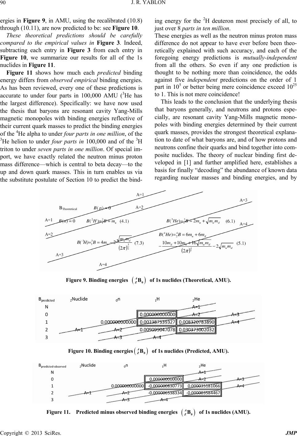

J. R. YABLON
JMP
90
er
w predict
eachtry in
Figure 10, we su
Figure 11 sh
d, every one o
re
ndent predictio
sonant cavity Yang-Mills magnetic mono-
poles with binding energies determined by their current
quark masses, provides the strongest theoretical explana-
tion to date of what baryons are, and of how prot
neutrons confine their quarks and bind together into com-
posite nuclides. The theory of nuclear binding first de-
ve
ing energy for the 2H deuteron most precisely of all, to
just over 8 parts in ten million.
These energies as well as the neutron minus proton mass
difference do not appear to have ever before been theo-
gies in Figure 9, in AMU, using the recalibrated (10.8)
through (10.11), are noed to be: see Figure 10.
These theoretical predictions should be carefully
compared to the empirical values in Figure 3. Indeed,
subtracting each entry in Figure 3 from en
mmarize our results for all of the 1s
nuclides in Figure 11.
ows how much each predicted binding
energy differs from observed empirical binding energies.
As has been reviewef these predictions is
accurate to under four parts in 100,000 AMU (3He has
the largest difference). Specifically: we have now used
the thesis that baryons are resonant cavity Yang-Mills
magnetic monopoles with binding energies reflective of
their current quark m
tically explained with such accuracy, and each of the
foregoing energy predictions is mutually-independent
from all the others. So even if any one prediction is
thought to be nothing more than coincidence, the odds
against five indepe ns on the order of 1
part in 105 or better being mere coincidence exceed 1025
to 1. This is not mere coincidence!
This leads to the conclusion that the underlying thesis
that baryons generally, and neutrons and protons espe-
cially, are re
asses to predict the binding energies
of the 4He alpha to under four parts in one million, of the
3He helion to under four parts in 100,000 and of the 3H
triton to under seven parts in one million. Of special im-
port, we have exactly related the neutron minus proton
mass difference—which is central to beta decay—to the
up and down quark masses. This in turn enables us via
the substitute postulate of Section 10 to predict the bind-
ons and
loped in [1] and further amplified here, establishes a
basis for finally “decoding” the abundance of known data
regarding nuclear masses and binding energies, and by
Figure 9. Binding energies


A
Z0
B of 1s nuclides (Theoretical, AMU).
Figure 10. Binding energies


o
A
Z0
Bf 1s nuclides (Predicted, AMU).
g energies


A
Z0
B of 1s nuclides (AMU). Figure 11. Predicted minus observed bindin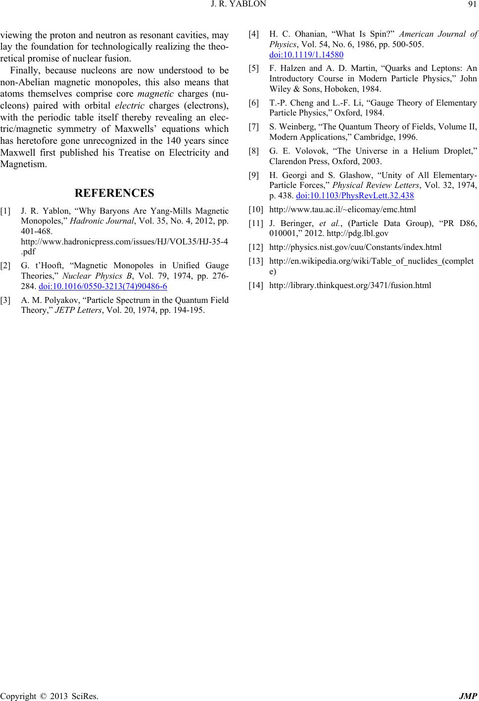

J. R. YABLON 91
agnetic charges (nu-
cl
has heretofore gone unrecognized in the 140 years since
Maxwell first published his Treatise on Electricity and
Magnetism.
REFERENCES
[1] J. R. Yablon, “Why Baryons Are Yang-Mills Magnetic
Monopoles,” Hadronic Journal, Vol. 35, No. 4, 2012, pp.
401-468.
http://www.hadronicpress.com/issues/HJ/VOL35/HJ-35-4
.pdf
[2] G. t’Hooft, “Magnetic Monopoles in Unified Gauge
Theories,” Nuclear Physics B, Vol. 79, 1974, pp. 276-
284. doi:10.1016/0550-
viewing the proton and neutron as resonant cavities, may
lay the foundation for technologically realizing the theo-
retical promise of nuclear fusion.
Finally, because nucleons are now understood to be
non-Abelian magnetic monopoles, this also means that
atoms themselves comprise core m
eons) paired with orbital electric charges (electrons),
with the periodic table itself thereby revealing an elec-
tric/magnetic symmetry of Maxwells’ equations which
3213(74)90486-6
[4] H. C. Ohanian, “What Is Spin?” American Journal of
Physics, Vol. 54, No. 6, 1986, pp. 500-505.
doi:10.1119/1.14580
[5] F. Halzen and A. D. Martin, “Quarks and Leptons: An
Introductory Course in Modern Particle Physics,” John
Wiley & Sons, Hoboken, 1984.
[6] T.-P. Cheng and L.-F. Li, “Gauge Theory of Elementary
Particle Physics,” Oxford, 1984.
[7] S. Weinberg, “The Quantum Theory of Fields, Volume II,
Modern Applications,” Cambridge, 1996.
[8] G. E. Volovok, “The Universe in a Helium Droplet,”
Clarendon Press, Oxford, 2003.
[9] H. Georgi and S. Glashow, “Unity of All Elementary-
Particle Forces,” Physical Review Letters, Vol. 32, 1974,
p. 438. doi:10.1103/PhysRevLett.32.438
[3] A. M. Polyakov, “Particle Spectrum in the Quantum Field
Theory,” JETP Letters, Vol. 20, 1974, pp. 194-195.
[10] http://www.tau.ac.il/~elicomay/emc.html
[11] J. Beringer, et al., (Particle Data Group), “PR D86,
010001,” 2012. http://pdg.lbl.gov
[12] http://physics.nist.gov/cuu/Constants/index.html
[13] http://en.wikipedia.org/wiki/Table_of_nuclides_(complet
e)
471/fusion.html [14] http://library.thinkquest.org/3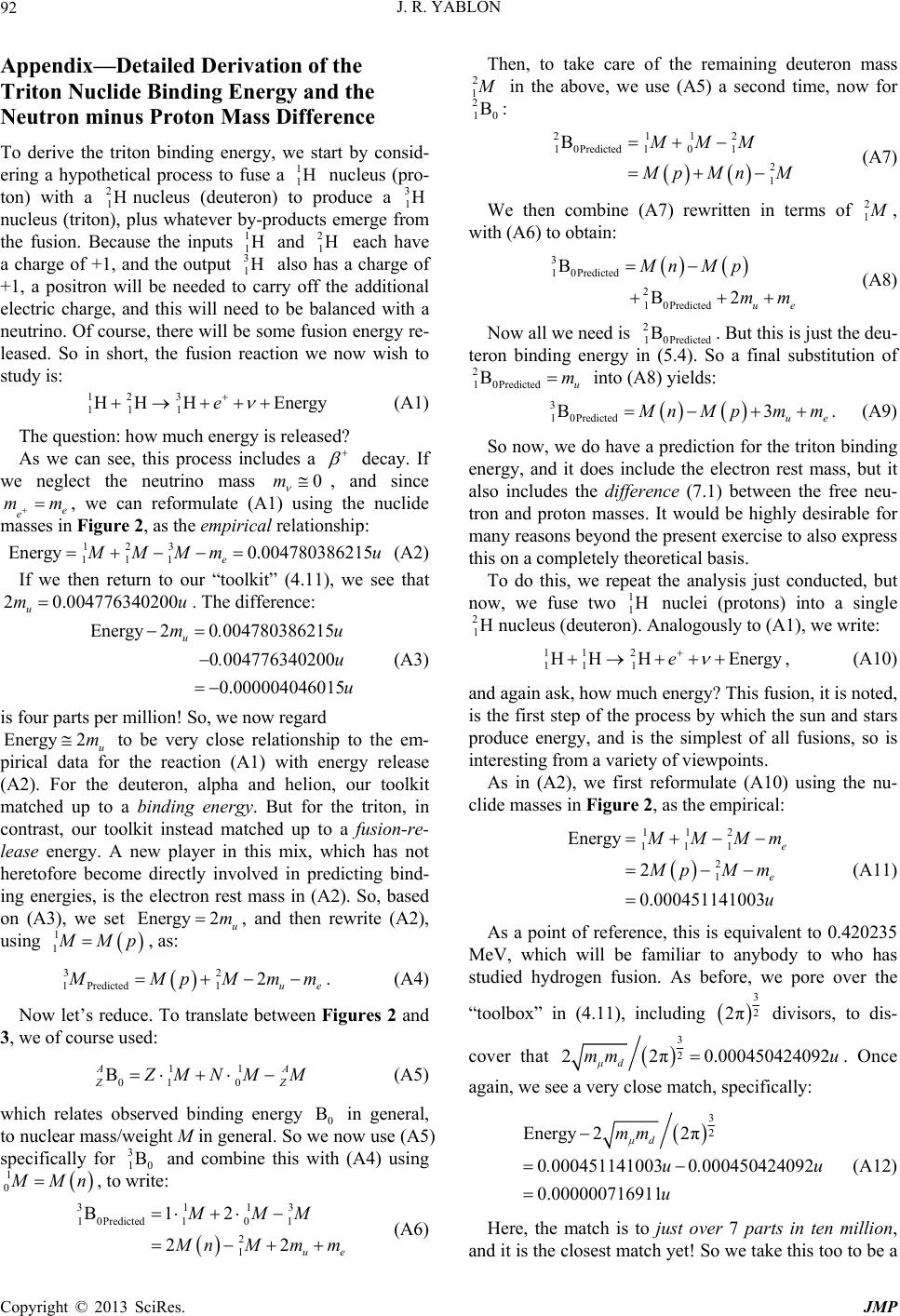

J. R. YABLON 92
Appendix—Detailed Derivation of the
Triton Nuclide Binding Energy and the
Neutron minus Proton Mass Difference
To derive the triton binding energy, we start by consid-
g a hypothetical process to fuserine a 1H nucleus (pro-
ton) with a 2
1Hnucleus (deuteron) to produce a 3 1H
leus (triton), plus whatever by-p
1
s a charge of
to be balanced with a
eutrino. Of course, there will be some fusion energy re-
ased. So in short, the fusion reaction we now wish to
udy is:
Energy   (A1)
The question: how much energy is released?
As we can see, this process icludes a
nuc roducts emerge from
the fusion. Because the inputs 1
1H and 2 1H each have
a charge of +1, and the output 3H also ha
1
+1 , a positron will be needed to carry off the additional
lectric charge, and this will neede
n
le
st
123
11 1
HH He 
n

 decay. If
e neglect the neutss 0m

, and since
e
e, we can rA1) using the nuclide
asses in Figure 2cal relationship:
4780386215
wrino
eformu
, as the
ma
late (
empiri
mm
m
123
111
Energy 0.00
e
M
MMm u (A2)
If we then return to our “toolkit” (4.11), we see that
76340200mu. The difference:
80386215
6340200
004046015
u
.u
u
(A3)
four parts per million! So, we now regard
ergy2 u m to be very close relationship to the em-
irical data for the reaction (A1) with energy release
2). For the deuteron, alpha and helion, our toolkit
atched up to a binding energy. But for the triton, in
ontrast, our toolkit instead matched up to a fusion-re-
ase energy. A new player in this mix, which has not
eretofore become directly involved in predicting bind-
g energies, is the electron rest mass in (A2). So, based
nEnergy2 u m, and then rewrite (A2),
2 0.0047
u
Energy20 0047
0 00477
0.000
u
m.


is
En
p
(A
m
c
le
h
in
o (A3), we set
ing

1
1
us
M
Mp, as:

32
1 Predicted12ue
M
MpMm m.
Now let’s reduce. To translate between Figures
3, we of course used:
(A4)
2 and
11
010
B
AA
ZZ
Z
MNM M (A5)
which relates observed binding energy 0 B in gene,
to nuclear mass/weight M in general. So we now use (A5)
specifically for 3
10
B and combi this with (A4) using

1
0
Then, to take care of the remaining deuteron mass
2
1
M
in the above, we use (A5) a second time, now for
2:
10
B
 
21

2
1
12
10Predicted1 0 1
BMMM
M
pMn

 (A7) M
2
We then combine (A7) rewritten in terms of 1
M
,
with (A6) to obtain:


3
1 0Predicted
BMnM p
2
10Predicted
B2
ue
mm

 (A8)
Now all we need is 2
1 0Predicted
B. But this is just the deu-
teron binding energy in (5.4). So a final substitution of
2
1 0Predicted
Bu m into (A8) yields:



3
1 0Predicted
B3
ue
M
nMp mm

. (A9)
So now, we do have a prediction for the triton binding
energy, and it does include the electron rest mass, but it
also includes the difference (7.1) between the free neu-
tron and proton masses. It would be highly desirable for
many reasons beyond the present exercise to also express
this on a completely theoretical basis.
To do this, we repeat the analysis just conducted, but
now, we fuse two 1
1H nuclei (protons) into a single
2
1Hnucleus (deuteron). Analogously to (A1), we write:
11 2
11 1
HH HEnergye 

 , (A10)
and again ask, how much energy? This fusion, it is noted,
is the first step of the process by which the sun and stars
produce energy, and is the simplest of all fusions, so is
interesting from a variety of viewpoints.
As in (A2), we first reformulate (A10) using the nu-
clide masses in Figure 2, as the empirical:

112
111
2
1
Energy
2
0.0004511410 03
e
e
M
MMm

M
pMm
u




(A11)
As a point of reference, this is equivalent to 0.420235
MeV, which will be familiar to anybody to who has
studied hydrogen fusion. As before, we pore over the
“toolbox” in (4.11), including

3
2
2π divisors, to dis-

ral
ne
M
Mn, to write:

3113
10Predicted 101
2
1
B12
22
ue
MMM
M
nMmm
 

(A6)
cover that
3
2
22π0.00045042
μd
mm 
ag
4092u. Once
ain, we see a very close match, specifically:

3
2
Energy 22π
0 0004511410030 000450424092
0.000000716911
μd
mm
.u.u
u



(A12) 
an
Here, the match is to just over 7 parts in ten million,
d it is the closest match yet! So we take this too to be a

J. R. YABLON 93
meaningful relationship, rite (A11) as: and use this to rew
 
2
1e
pM m.
Now we need to reduce this expression. First, using
2
3
2
22π2
μd
mm M (A13)
(4.1), namely 10 Bu m, we write (A7) as:



2
1u
M
MpMn m. (A14)
Then we combine (A14) with (A13) and rearrange,
and also use (1.11), to obtain the prediction:
 



Predicted
3
2
3
2
22π
33 2π
16609
ue μd
uu
MnM p
mm mm
mmm
 


 
(A15)
2
0.001389 9
dμd
mm
u


This is an extremely important relatio
th
nship relating
e observed difference (7.1) between the neutron and
proton mass
 
0.001388449188
M
nMp u solely
to the up and down (and optionally electron) rest masses.
This is useful in a wide array of circu
cially between nuclear isobars (along the diagonal lines
he
mstances, espe-
of like-A which are shown in the figures re) which by
definition convert into one another via beta decay. Com-
paring (A15) with (7.1), we see that:
 


Observed
9188
M p
u



A
thisy
empirical data.
Because of this, we now take (A15) to b
Predicted
0 0013891660990 00138844
0.000000716911
MnM pMn
.u.
u
 



(A16)
This is the exact same degree of accuracy, to just over
7 parts in ten millionMU, which we saw in (A12). So
is yet another relationship matched very closely b
e a meaningful
relationship, and use this in (A9) to write:



33
010Predicted
Predicted
BH B
3
As a result, we finally have a theoretical expression
for the binding energy of the triton, totally in term
up and down quark masses. The empirica
2
42 2π
0.009102256308
uμd
mmm
u


(A17)
s of the
l value 3
10
B

0.009105585412u is shown in Figure 3, and doing the
co
00332
just ove
illion AMU!
mparison, we have:
33
1 0Predicted1 0
BB 0.009102256308
0.009105585 412
u
u

 (A18)
0.000 9104u
We see that this result is accurate to r three
parts in one m