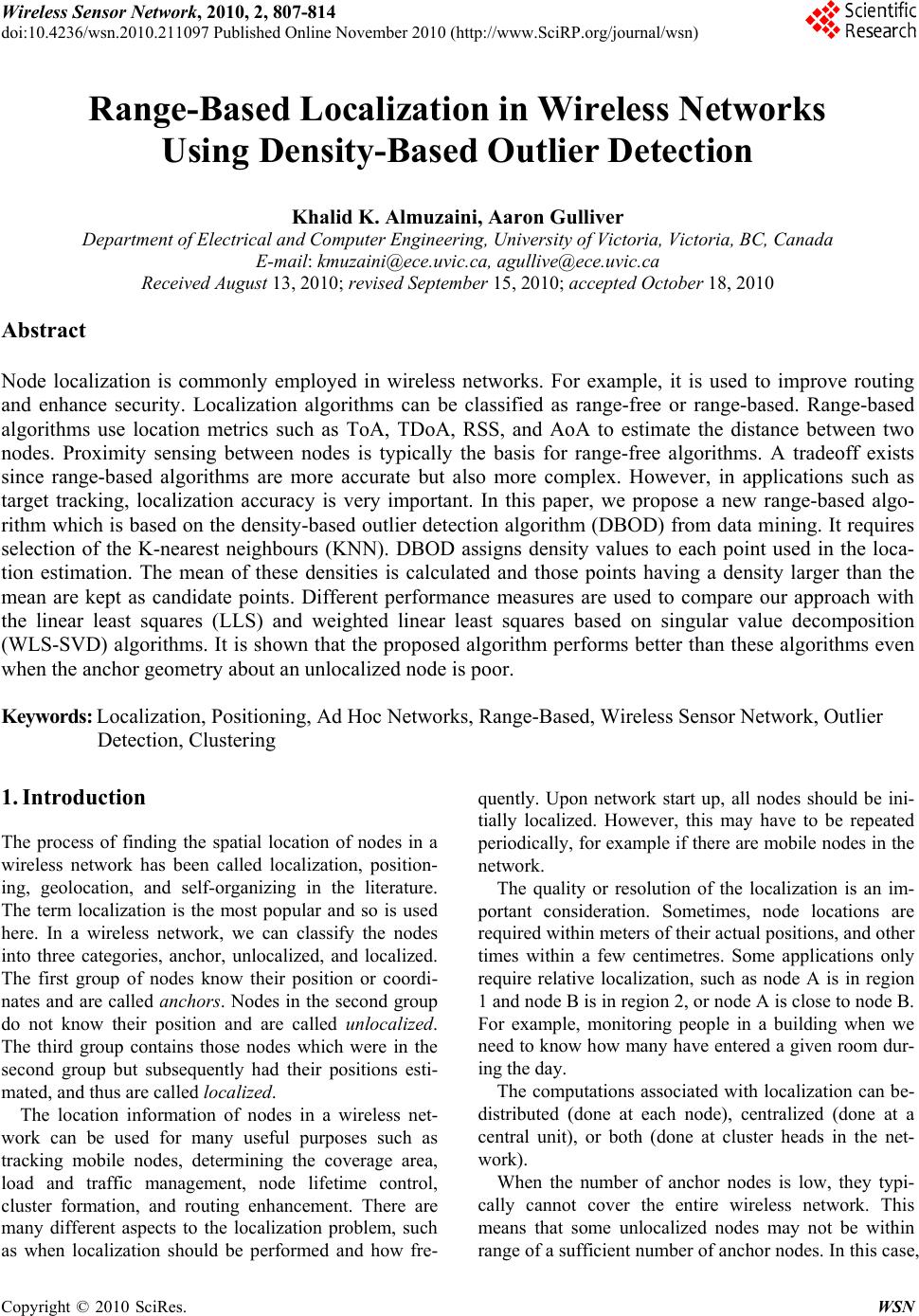Wireless Sensor Network, 2010, 2, 807-814
doi:10.4236/wsn.2010.211097 Published Online November 2010 (http://www.SciRP.org/journal/wsn)
Range-Based Localization in Wireless Networks
Using Density-Based Outlier Detection
Khalid K. Almuzaini, Aaron Gulliver
Department of Electrical and Computer Engineering, University of Victoria, Victoria, BC, Canada
Received August 13, 2010; revised September 15, 2010; accepted October 18, 2010
Abstract
Node localization is commonly employed in wireless networks. For example, it is used to improve routing
and enhance security. Localization algorithms can be classified as range-free or range-based. Range-based
algorithms use location metrics such as ToA, TDoA, RSS, and AoA to estimate the distance between two
nodes. Proximity sensing between nodes is typically the basis for range-free algorithms. A tradeoff exists
since range-based algorithms are more accurate but also more complex. However, in applications such as
target tracking, localization accuracy is very important. In this paper, we propose a new range-based algo-
rithm which is based on the density-based outlier detection algorithm (DBOD) from data mining. It requires
selection of the K-nearest neighbours (KNN). DBOD assigns density values to each point used in the loca-
tion estimation. The mean of these densities is calculated and those points having a density larger than the
mean are kept as candidate points. Different performance measures are used to compare our approach with
the linear least squares (LLS) and weighted linear least squares based on singular value decomposition
(WLS-SVD) algorithms. It is shown that the proposed algorithm performs better than these algorithms even
when the anchor geometry about an unlocalized node is poor.
Keywords: Localization, Positioning, Ad Hoc Networks, Range-Based, Wireless Sensor Network, Outlier
Detection, Clustering
1. Introduction
The process of finding the spatial location of nodes in a
wireless network has been called localization, position-
ing, geolocation, and self-organizing in the literature.
The term localization is the most popular and so is used
here. In a wireless network, we can classify the nodes
into three categories, anchor, unlocalized, and localized.
The first group of nodes know their position or coordi-
nates and are called anchors. Nodes in the second group
do not know their position and are called unlocalized.
The third group contains those nodes which were in the
second group but subsequently had their positions esti-
mated, and thus are called localized.
The location information of nodes in a wireless net-
work can be used for many useful purposes such as
tracking mobile nodes, determining the coverage area,
load and traffic management, node lifetime control,
cluster formation, and routing enhancement. There are
many different aspects to the localization problem, such
as when localization should be performed and how fre-
quently. Upon network start up, all nodes should be ini-
tially localized. However, this may have to be repeated
periodically, for example if there are mobile nodes in the
network.
The quality or resolution of the localization is an im-
portant consideration. Sometimes, node locations are
required within meters of their actual positions, and other
times within a few centimetres. Some applications only
require relative localization, such as node A is in region
1 and node B is in region 2, or no de A is close to nod e B.
For example, monitoring people in a building when we
need to know how many have entered a given room dur-
ing the day.
The computations associated with localization can be-
distributed (done at each node), centralized (done at a
central unit), or both (done at cluster heads in the net-
work).
When the number of anchor nodes is low, they typi-
cally cannot cover the entire wireless network. This
means that some unlocalized nodes may not be within
range of a sufficient number of anchor nodes. In this case,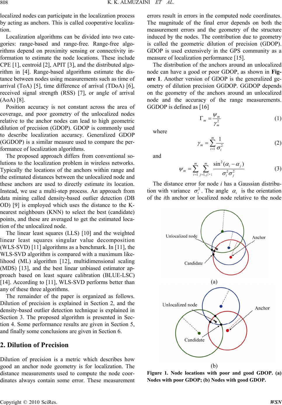

K. K. ALMUZAINI ET AL. 808
localized nodes can participate in the localization process
by acting as anchors. This is called cooperative localiza-
tion.
Localization algorithms can be divided into two cate-
gories: range-based and range-free. Range-free algo-
rithms depend on proximity sensing or connectivity in-
formation to estimate the node locations. These include
CPE [1], centro id [2], APIT [3], an d the distribu ted algo-
rithm in [4]. Range-based algorithms estimate the dis-
tance between nodes using measurements such as time of
arrival (ToA) [5], time difference of arrival (TDoA) [6],
received signal strength (RSS) [7], or angle of arrival
(AoA) [8].
Position accuracy is not constant across the area of
coverage, and poor geometry of the unlocalized nodes
relative to the anchor nodes can lead to high geometric
dilution of precision (GDOP). GDOP is commonly used
to describe localization accuracy. Generalized GDOP
(GGDOP) is a similar measure used to compare the per-
formance of localization algorithms.
The proposed approach differs from conventional so-
lutions to the localization problem in wireless networks.
Typically the locations of the anchors within range and
the estimated distances between the unlocalized node and
these anchors are used to directly estimate its location.
Instead, we use a multi-step process. An approach from
data mining called density-based outlier detection (DB
OD) [9] is employed which uses the distance to the K-
nearest neighbours (KNN) to select the best (candidate)
points, and these are averaged to get the estimated loca-
tion of the unlocalized node.
The linear least squares (LLS) [10] and the weighted
linear least squares singular value decomposition
(WLS-SVD) [11] algorithms as a benchmark. In [11], the
WLS-SVD algorithm is compar ed wit h a max imum l ike-
lihood (ML) algorithm [12], multidimensional scaling
(MDS) [13], and the best linear unbiased estimator ap-
proach based on least square calibration (BLUE-LSC)
[14]. According to [11], WLS-SVD performs better than
any of these three algorithms.
The remainder of the paper is organized as follows.
Dilution of precision is explained in Section 2, and the
density-based outlier detection technique is explained in
Section 3. The proposed algorithm is presented in Sec-
tion 4. Some performance results are given in Section 5,
and finally some conclusions are given in Section 6.
2. Dilution of Precision
Dilution of precision is a metric which describes how
good an anchor node geometry is for localization. The
distance measurements used to compute the node coor-
dinates always contain some error. These measurement
errors result in errors in the computed node coordinates.
The magnitude of the final error depends on both the
measurement errors and the geometry of the structure
induced by the nodes. The contribution due to geometry
is called the geometric dilution of precision (GDOP).
GDOP is used extensively in the GPS community as a
measure of localization performance [15].
The distribution of the anchors around an unlocalized
node can have a good or poor GDOP, as shown in Fig-
ure 1. Another version of GDOP is the generalized ge-
ometry of dilution precision GGDOP. GGDOP depends
on the geometry of the anchors around an unlocalized
node and the accuracy of the range measurements.
GGDOP is defined as [16]
2
m
m
m


 (1)
where
2
1
1
m
mii





(2)
and 2
22
11,
sin ()
mm ij
mijj ij






＞i
(3)
The distance error for node i has a Gaussian distribu-
tion with variance 2
i

. The angle i

is the orientation
of the ith anchor or localized node relative to the node
(a)
(b)
Figure 1. Node locations with poor and good GDOP. (a)
Nodes with poor GDOP; (b) Nodes with good GDOP.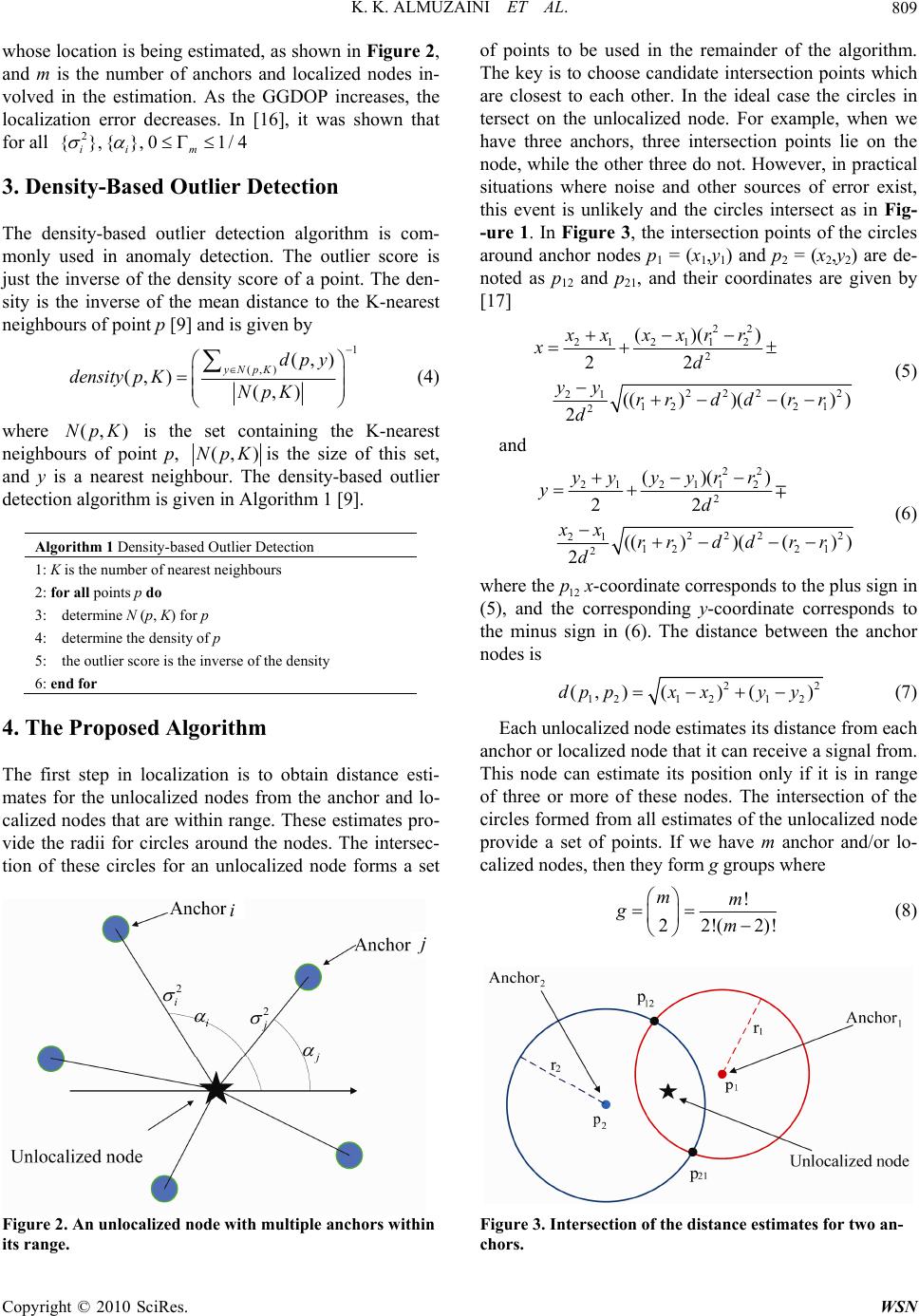

K. K. ALMUZAINI ET AL. 809
whose location is being estimated, as shown in Figure 2,
and m is the number of anchors and localized nodes in-
volved in the estimation. As the GGDOP increases, the
localization error decreases. In [16], it was shown that
for all 2
{},{},0 1/4
ii m
  
3. Density-Based Outlier Detection
The density-based outlier detection algorithm is com-
monly used in anomaly detection. The outlier score is
just the inverse of the density score of a point. The den-
sity is the inverse of the mean distance to the K-nearest
neighbours of point p [9] and is given by
1
(,) (,)
(, )(, )
yNpKdpy
densityp KNpK






 (4)
where (, )NpK is the set containing the K-nearest
neighbours of point p, (, )NpKis the size of this set,
and y is a nearest neighbour. The density-based outlier
detection algorith m is given in Algorithm 1 [9].
Algorithm 1 Density-based Outlier Detection
1: K is the number of nearest neighbours
2: for all points p do
3: determine N (p, K) for p
4: determine the density of p
5: the outlier score is the inverse of the density
6: end for
4. The Proposed Algorithm
The first step in localization is to obtain distance esti-
mates for the unlocalized nodes from the anchor and lo-
calized nodes that are within range. These estimates pro-
vide the radii for circles around the nodes. The intersec-
tion of these circles for an unlocalized node forms a set
Figure 2. An unlocalized node with multiple anchors within
its range.
of points to be used in the remainder of the algorithm.
The key is to choose candidate intersection points which
are closest to each other. In the ideal case the circles in
tersect on the unlocalized node. For example, when we
have three anchors, three intersection points lie on the
node, while the other three do not. However, in practical
situations where noise and other sources of error exist,
this event is unlikely and the circles intersect as in Fig-
-ure 1. In Figure 3, the intersection points of the circles
around anchor nodes p1 = (x1,y1) and p2 = (x2,y2) are de-
noted as p12 and p21, and their coordinates are given by
[17]
22
21211 2
2
222 2 21 12 21
2
()()
22
(())(() )
2
xx xxrr
xd
yy rrddrr
d

 
 
(5)
and
22
21 2112
2
222 2
21 12 21
2
()()
22
(())(())
2
yy yyrr
yd
xx rrddrr
d


 

(6)
where the12 px-coordinate corresponds to the plus sign in
(5), and the corresponding y-coordinate corresponds to
the minus sign in (6). The distance between the anchor
nodes is
22
121 212
(, )()()dp pxxyy (7)
Each unlocalized node estimates its distance from each
anchor or localized node that it can receive a signal from.
This node can estimate its position only if it is in range
of three or more of these nodes. The intersection of the
circles formed from all estimates of the unlocalized node
provide a set of points. If we have m anchor and/or lo-
calized nodes, then they form g groups where
!
22!( 2)!
mm
gm


 
 (8)
Figure 3. Intersection of the distance estimates for two an-
chors.
2
i

i

2
j

j

i
j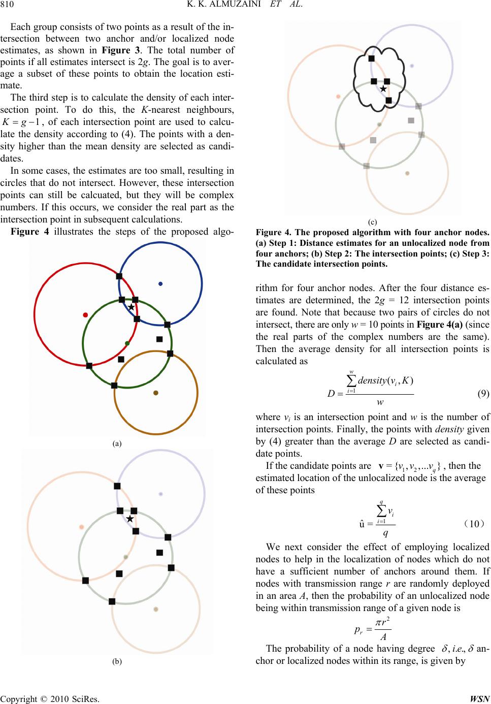

K. K. ALMUZAINI ET AL. 810
Each group consists of two points as a result of the in-
tersection between two anchor and/or localized node
estimates, as shown in Figure 3. The total number of
points if all estimates intersect is 2g. The goal is to aver-
age a subset of these points to obtain the location esti-
mate.
The third step is to calculate the density of each inter-
section point. To do this, the K-nearest neighbours,
1Kg , of each intersection point are used to calcu-
late the density according to (4). The points with a den-
sity higher than the mean density are selected as candi-
dates.
In some cases, the estimates are too small, resulting in
circles that do not intersect. However, these intersection
points can still be calcuated, but they will be complex
numbers. If this occurs, we consider the real part as the
intersection point in subsequent calculations.
Figure 4 illustrates the steps of the proposed algo-
(a)
(b)
(c)
Figure 4. The proposed algorithm with four anchor nodes.
(a) Step 1: Distance estimates for an unlocalized node from
four anchors; (b) Step 2: The intersection points; (c) Step 3:
The candidate intersection points.
rithm for four anchor nodes. After the four distance es-
timates are determined, the 2g = 12 intersection points
are found. Note that because two pairs of circles do not
intersect, there are only w = 10 points in Figure 4(a) (since
the real parts of the complex numbers are the same).
Then the average density for all intersection points is
calculated as
1
(, )
w
i
i
density vK
Dw

 (9)
where vi is an intersection point and w is the number of
intersection points. Finally, the points with density given
by (4) greater than the average D are selected as candi-
date points.
If the candidate points are 12 = {,,...}
q
vv vv, then the
estimated location of the unlocalized node is the average
of these points
1
ˆ
u=
q
i
i
v
q

 （10）
We next consider the effect of employing localized
nodes to help in the localization of nodes which do not
have a sufficient number of anchors around them. If
nodes with transmission range r are randomly deployed
in an area A, then the probability of an unlocalized node
being within transm ission ran ge of a give n node is
2
rr
p
A


The probability of a node having degree ,..,ie


an-
chor or localized nodes within its range, is given by

K. K. ALMUZAINI ET AL. 811
() ! Pe






where
r
Np


and N is the number of anchor and localized nodes. Then
the probability of a node having n or more anchor and
localized nodes within its range is
1
()1 ()
n
io
pn pi 




5. Performance Results
In this section, the proposed algorithm LDBOT is com-
pared with the WLS-SVD [11] and LLS [10] algorithms
via simulation. We first consider distance to measure the
accuracy of both techniques. 100 nodes are deployed,
50% of which are anchors which are chosen randomly.
The deployment area is A = 100 × 100 m2, and the range
is r = 10 m. The distance error has a Gaussian distribu-
tion with variance 2
d

which is a percentage of the ac-
tual distance. As a performance measure, we use the
mean error, which is defined as
22
1
ˆˆ ()()
meanerror
u
ii ii
ti
x
xyy
tu


 (11)
where u is the number of unlocalized nodes, t is the
number of trials, ˆˆ
(, )
x
y is the estimated unlocalized node
position, and (x, y) is the actual position. The results
were ave rag ed o ver 10 4 trials. Localized nodes wer e used
with the anchors to localize those unlocalized nodes
which were not within range of a sufficient number of
anchor and localized nodes in the previous iterations.
The localization process ends when all nodes are lo-
calized or all remaining unlocalized nodes are isolated,
i.e., not within range of three or more anchor or localized
nodes. Figure 5 shows that the mean error with the pro-
posed algorithm outperforms that with the LLS and
Figure 5. Mean error versus distance variance.
WLS-SVD algortihms. Note that the rate of change of
the error is also lower with LDBOD.
Next all algorithms are compared considering the trans-
mission range of the wireless nodes. The deployment
area, the number of nodes, and the number of an chor s ar e
the same as before but the transmission range varies from
10 m to 50 m. The distance error variance is fixed at 10%
of the actual distance between nodes. The results were
again averaged over 104 trials. Figure 6 shows that the
proposed algorithm performs better than the LLS and
WLS-SVD algorithms at low transmission ranges, in
which case the unlocalized nodes are typically within
range of a small number of nodes. However, at high
transmission ranges all algorithms have similar per-
formance.
The probability that an unlocalized node has 3 or more
anchor or localized nodes around it based on a given
transmission range is illustrated in Figure 7. This clearly
Figure 6. Mean error versus transmission range.
Figure 7. Probability of node localization based on trans-
mission range.

K. K. ALMUZAINI ET AL. 812
shows that using localized nodes in the localization
process improves the probability of localizing nodes.
When the range exceeds 25 m, all unlocalized nodes can
be localized.
The anchor ratio is one of the most important factors
affecting localization accuracy. Thus we next compare-
the algorithms with a varying percentage of anchor nodes.
In this case we are more interested in the performance
when the anchor ratio is small because in a practical sys-
tem the number of anchor nodes will be much lower than
the number of unlocalized nodes. The deployment area
and the number of nodes are the same as before but the
anchor ratio varies from 20% to 80%. The transmission
range is fixed at 10 m and the distance error variance is
fixed at 10% of the actual distance. The results are again
averaged over 104 trials. Figure 8 shows that the pro-
posed algorithm again outperforms both the LLS and
WLS-SVD algorithms, particularly at low anchor ratios.
The probability that an unlocalized node has 3 or more
anchor or localized nodes around it based on a given
anchor ratio is shown in Figure 9. Clearly the use of
Figure 8. Mean error versus anchor ratio.
Figure 9. Probability of node localization based on the an-
chor ratio.
localized nodes in the localization process improve the
probability of node localization. This probability reaches
a maximum of only 0.6 due to the small range of 10 m.
Next we consider the effect of the node geometry on
performance, with GGDOP used as the geometry meas-
-ure. Three anchor nodes are deployed on a circle with a
fourth unlocalized node in the center. The transmission
range is set to 30 m to ensure that the unlocalized node is
within range of the three anchors, and the distance error
variance is set to 10%. The anchors a1, a2, and a3 are
distributed around the unlocalized node u at angles
12
aua and 23 aua ranging from 1˚ to 101˚ (with
both angles the same). The results are averaged over 104
trials, and are shown in Figure 10 for GGDOP and in
Figure 11 for angle between anchors. Both figures show
that the proposed algorithm performs better, particularly
when the geometry is poor, i.e., low GGDOP or small
angles. The LLS and WLS-SVD algorithms perform
similarly at all angles and GGDOP values because only
Figure 10. Mean error versus GGDOP.
Figure 11. Mean error versus angle between anchors.

K. K. ALMUZAINI ET AL. 813
(a)
(b)
(c)
Figure 12.Mean error surfaces. (a) Mean error surface for
the LLS algorithm; (b) Mean error surface for the
WLS-SVD algorithm; (c) Mean error surface for the
LDBOD algorithm.
four nodes are deployed. At small angles, the geometry is
poor, and as the angles increase the geometry approaches
the ideal case where the anchors are distributed uniformly
on the circle. Thus at angles of 101˚ the performance is
very good, and all three algorithms perform similarly.
Finally, we evaluated the algorithms with different
anchor ratios and distance error variances. Figure 12
shows the resulting mean error surfaces. Clearly LDBOD
outperforms the other algorithms at high distance error
variances (90%) and low anchor ratios (10%), which is
the most typical, but also the most challenging environ-
ment. The performance is similar at high anchor ratios
(90%) and low distance error variances (10%), which is
close to the ideal case, and therefore not likely to occur
in practice.
6. Conclusions
A new range-based localization algorithm (LDBOD) has
been presented which is based on the density-based out-
lier detection (DBOD) algorithm, a concept from data
mining. The proposed algorithm is used to select the best
points (candidates) from a set of distance estimate inter-
section points. The proposed algorithm was shown to
outperform the LLS and recently proposed WLS-SVD
algorithms.
7. References
[1] L. Doherty, K. S. J. Pister and L. El Ghaoui, “Convex
Position Estimation in Wireless Sensor Networks,” Pro-
ceedings of IEEE INFOCOM, Anchorage, AK, April
2001, pp. 1655-1663.
[2] N. Bulusu, J. Heidemann and D. Estrin, “GPS-Less
Low-Cost Outdoor Localization for Very Small Devices,”
IEEE Personal Communications, Vol. 7, No. 5, October
2000, pp. 28-34.
[3] T. He, C. Huang, B. M. Blum, J. A. Stankovic and T.
Abdelzaher, “Range-Free Localization Schemes For Large
Scale Sensor Networks,” Proceedings of ACM MobiCom,
San Diego, CA, September 2003, pp. 81-95.
[4] K. Almuzaini and T. A. Gulliver, “A New Distributed
Range-Free Localization Algorithm for Wireless Net-
works,” Proceedings of IEEE Vehicular Technology
Conference, Anchorage, AK, September 2009, pp. 20-23.
[5] I. Guvenc and Z. Sahinoglu, “Threshold-Based TOA
Estimation for Impulse Radio UWB Systems,” Proceed-
ings of IEEE International Conference on Ultra-Wideband,
Zurich, Switzerland, September 2005, pp. 420-425.
[6] X. Wei, L. Wa ng and J. Wan, “A New Loc alization Tech-
nique Based on Network TDOA Information,” Proceed-
ings of IEEE International Conference on ITS Telecom-
munications, Chengdu, China, June 2006, pp. 127-130.
[7] A. Hatami, K. Pahlavan, M. Heidari and F. Akgul, “On
RSS and TOA Based Indoor Geolocation—A Compara-

K. K. ALMUZAINI ET AL. 814
tive Performance Evaluation,” Proceedings of IEEE
Wireless Communications and Networking Conference,
Las Vegas, NV, April 2006, pp. 2267-2272.
[8] D. Niculescu and B. Nath, “Ad Hoc Positioning System
(APS) Using AOA,” Proceedings of IEEE INFOCOM,
San Francisco, CA, March-April 2003, pp. 1734-1743.
[9] P. N. Tan, M. Steinbach and V. Kumar, “Introduction to
Data Mining,” Pearson Addison Wesley, Boston, 2006.
[10] I. Guvenc, C.-C. Chong and F. Watanabe, “Analysis of a
Linear Least-Squares Localization Technique in LOS and
NLOS Environments,” Proceedings of IEEE Vehicular
Technology Conference, Dublin, Ireland, April 2007, pp.
1886-1890.
[11] C.-H. Park and K.-S. Hong, “Source Localization Based
on SVD without a Priori Knowledge,” Proceedings of
IEEE International Conference on Advanced Communi-
cations Technology, Phoenix Park, Korea, February 2010,
pp. 3-7.
[12] D. J. Torrieri, “Statistical Theory of Passive Location
Systems,” IEEE Transactions on Aerospace and Elec-
tronic Systems, Vol. 20, No. 2, March 1984, pp. 183-198.
[13] H. C. So and F. K. W. Chan, “A Generalized Subspace
Approach for Mobile Positioning with Time-of-Arrival
Measurements,” IEEE Transactions on Signal Processing,
Vol. 55, No. 10, October 2007, pp. 5103-5107.
[14] F. K. W. Chan, H. C. So, J. Zheng and K. W. K. Lui,
“Best Linear Unbiased Estimator Approach for Time-
of-Arrival Based Localisation,” IET Signal Processing,
Vol. 2, No. 2, June 2008, pp.156-163.
[15] D. B. Jourdan, D. Dardari and M. Z. Win, “Position Error
Bound for UWB Localization in Dense Cluttered Envi-
ronments,” Proceedings of IEEE International Confer-
ence on Communications, Istanbul, Turkey, June 2006,
pp. 3705-3710.
[16] S. Venkatesh and R. M. Buehrer, “Multiple-Access De-
sign for Ad Hoc UWB Position-Location Networks,” Pro-
ceedings of IEEE Wireless Communications and Net-
working Conference, Las Vegas, NV, April 2006, pp.
1866-1873.
[17] J. Vince, “Geometry for Computer Graphics: Formulae,
Examples and Proofs,” Springer, Berlin, 2005.