J. Software Engi neeri n g & Applications, 2010, 3, 906-913
doi:10.4236/jsea.2010.310107 Published Online October 2010 (http://www.SciRP.org/journal/jsea)
Accuracy of Measuring Camera Position by
Marker Observation
Vladimir A. Grishin
Space Research Institute (IKI), Russian Academy of Sciences, Moscow, Russia.
Received July 14th, 2010; revised August 10th, 2010; accepted August 14th, 2010.
ABSTRACT
A lower bound to errors of measuring object position is constructed as a function of parameters of a monocular com-
puter vision system (CVS) as well as of observation cond itions and a shape of an observed marker. Th is bound justifies
the specification of the CVS parameters and allows us to formulate constraints for an object trajectory based on re-
quired measu r ement accuracy. For making the measure ment, the boundaries of marker image are used.
Keywords: Computer Vision System, Camera Position Measurement, Marker Observation, Lower Bound to Errors
1. Introduction
CVSs are widely applied for a solution of motion control
problems. This fact is associated by the following condi-
tions. First, the computational capability of available
processors allows for the real-time processing of large
volumes of information formed by TV cameras. The in-
formation processing time proves to be acceptable to a
number of practical problems [1-6]. Second, the increas-
ing application of computer-aided control systems of
unmanned aerial vehicles requires the enhancement of
the vector of measured parameters to solve the automatic
landing problem [5]. Another task is a docking problem
(including the spacecraft docking), which requires pre-
cise measuring a relative position for solving the terminal
control task [6]. As an example we can refer to the dock-
ing the first European Automated Transfer Vehicle (ATV)
“Jules Verne” to the International Space Station (ISS) on
3 April 2008. In the above experiment, a special com-
puter vision system was used for measuring the relative
spatial and angular position.
All of these facts stimulate interest in estimation of the
potential accuracy (lower bounds to errors) of measuring
the position parameters as a function of the marker shape,
its observation condition and technical parameters of the
CVS. This allows us to evaluate an applicability of CVSs
to solving control problems under specific conditions as
well as to optimize the CVS parameters from the view-
point of ensuring the required accuracy of measurements.
There are a small number of publications devoted to the
problems of determining the current coordinates meas-
urement precision estimation. Most publications are
based on experimental approach (full-scale experiments
or stochastic simulation) to the measurement precision
estimation. For obtaining reliable estimation, such ap-
proach requires too much time and additionally the
full-scale experiments are very expensive.
In [7], the Cramér–Rao bound is constructed to camera
position estimation by docking marker observation. For
position estimation, a set of the marker features (points
of interest) are used, namely corners, contrast spots and
others. This approach is suitable for the case of small or
medium marker observation distance. In such distances
the visible size of marker is of order tens or hundreds of
pixels in any direction. In the present paper, we consider
the approach, which is suitable for large distances by
using the boundaries between marker image and back-
ground. This approach allows obtaining lower bound to
errors of measuring object position with small computa-
tional expenses. It allows in one’s turn to optimize CVS
parameters and marker shape for a specified set of the
observation conditions.
In Section 2, we formulate the assumptions for con-
structing the bound to errors. In Section 3, we construct a
Cramér–Rao bound to the measurement errors and, in
Section 4, we present experimental results.
2. Assumptions Made When Constructing a
Bound
We make the following simplifying assumptions to esti-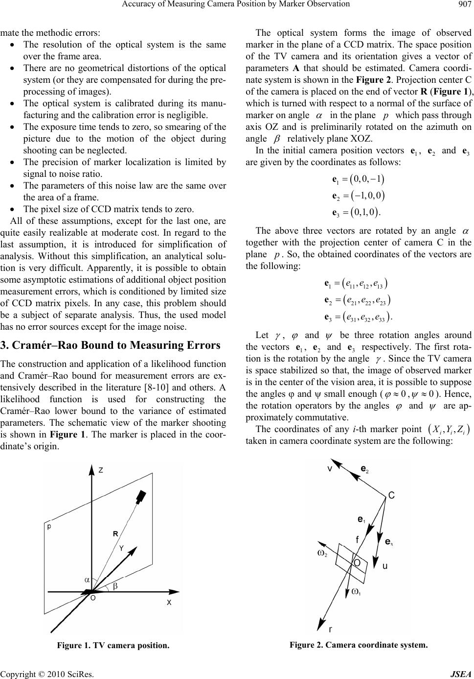

Accuracy of Measuring Camera Position by Marker Observation907
mate the methodic errors:
 The resolution of the optical system is the same
over the frame area.
 There are no geometrical distortions of the optical
system (or they are compensated for during the pre-
processing of images).
 The optical system is calibrated during its manu-
facturing and the calibration error is negligible.
 The exposure time tends to zero, so smearing of the
picture due to the motion of the object during
shooting can be neglected.
 The precision of marker localization is limited by
signal to noise ratio.
 The parameters of this noise law are the same over
the area of a frame.
 The pixel size of CCD matrix tends to zero.
All of these assumptions, except for the last one, are
quite easily realizable at moderate cost. In regard to the
last assumption, it is introduced for simplification of
analysis. Without this simplification, an analytical solu-
tion is very difficult. Apparently, it is possible to obtain
some asymptotic estimations of additional object position
measurement errors, which is conditioned by limited size
of CCD matrix pixels. In any case, this problem should
be a subject of separate analysis. Thus, the used model
has no error sources except for the image noise.
3. Cramér–Rao Bound to Measuring Errors
The construction and application of a likelihood function
and Cramér–Rao bound for measurement errors are ex-
tensively described in the literature [8-10] and others. A
likelihood function is used for constructing the
Cramér–Rao lower bound to the variance of estimated
parameters. The schematic view of the marker shooting
is shown in Figure 1. The marker is placed in the coor-
dinate’s origin.
Figure 1. TV camera position.
The optical system forms the image of observed
marker in the plane of a CCD matrix. The space position
of the TV camera and its orientation gives a vector of
parameters A that should be estimated. Camera coordi-
nate system is shown in the Figure 2. Projection center C
of the camera is placed on the end of vector R (Figure 1),
which is turned with respect to a normal of the surface of
marker on angle

in the plane which pass through
axis OZ and is preliminarily rotated on the azimuth on
angle
p

relatively plane XOZ.
In the initial camera position vectors , and
are given by the coordinates as follows:
1
e2 e3 e




1
2
3
0, 0,1
1, 0,0
0,1,0.




e
e
e
The above three vectors are rotated by an angle

together with the projection center of camera C in the
plane . So, the obtained coordinates of the vectors are
the following:
p




1111213
2212223
3313233
,,
,,
,,
eee
eee
eee



e
e
e.
Let

,

and

be three rotation angles around
the vectors 1, 2 and 3
e respectively. The first rota-
tion is the rotation by the angle
e e

. Since the TV camera
is space stabilized so that, the image of observed marker
is in the center of the vision area, it is possible to suppose
the angles  and  small enough (0

,0

). Hence,
the rotation operators by the angles

and

are ap-
proximately commutative.
The coordinates of any i-th marker point


,,
ii i
X
YZ
taken in camera coordinate system are the following:
Figure 2. Camera coordinate system.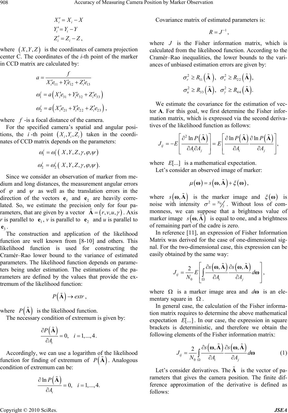

Accuracy of Measuring Camera Position by Marker Observation 908
,
ii
ii
ii
X
XX
YYY
Z
ZZ



where

,,

X
YZ is the coordinates of camera projection
center C. The coordinates of the i-th point of the marker
in CCD matrix are calculated by:
11 1213ii i
f
a
X
eYeZe



13132
iii i
aXeYeZe 


33

23

22122
iii i
aXeYeZe 

 ,
where
f
-is a focal distance of the camera.
For the specified camera’s spatial and angular posi-
tions, the i-th point

,,
ii i
X
YZ taken in the coordi-
nates of CCD matrix depends on the parameters:

11,,,,,
ii
XYZ





22
,,,,, .
ii
XYZ




Since we consider an observation of marker from me-
dium and long distances, the measurement angular errors
of

and

as well as the translation errors in the
direction of the vectors 3 and 2 are heavily corre-
lated. So, we estimate the precision only for four pa-
rameters, that are given by a vector
e e

,,,rvu

A

2
e
. Axis
r is parallel to , v is parallel to and u is parallel to
.
1
e
3
e
The construction and application of the likelihood
function are well known from [8-10] and others. This
likelihood function is used for constructing the
Cramér–Rao lower bound to the variance of estimated
parameters. The likelihood function depends on parame-
ters being under estimation. The estimations of the pa-
rameters are defined by the values that provide the ex-
tremum of the likelihood function:

P extrA
,
where is the likelihood function.

PA

The necessary condition of extremum is given by:

0,1,..., 4.
i
Pi
A


A

Accordingly, we can use a logarithm of the likelihood
function for finding of extremum of . Analogous
condition of extremum can be:

PA


ln 0,1,..., 4.
i
Pi
A


A

Covariance matrix of estimated parameters is:
1
RJ

,
where
J
is the Fisher information matrix, which is
calculated from the likelihood function. According to the
Cramér–Rao inequalities, the lower bounds to the vari-
ances of unbiased estimation errors are given by:


22
112 2
,,
rv
RR  AA




22
33 44
,.
uRR 
 AΑ


We estimate the covariance for the estimation of vec-
tor A. For this goal, we first determine the Fisher infor-
mation matrix, which is expressed via the second deriva-
tives of the likelihood function as follows:




2lnln ln
,
ij iji j
PPP
JE E
AAA A

 


 
 
 

 

 
AA

A

where is a mathematical expectation.
[...]E
Let’s consider an observed image of marker:




,s  ωωAω
,
where


,sωA
 is the marker image and


 ω is
noise with intensity 0
2
2
N
 . Without loss of com-
monness, we can suppose that a brightness value of
marker image


,ωA

s is equal to one, and a brightness
of remaining part of the cadre is zero.
In reference [11], an expression of Fisher Information
Matrix was derived for the case of one-dimensional sig-
nal. For the two-dimensional case, this expression can be
easily obtained by the same way:


0
,,
2
ij ij
ss
J
Ed
NAA











ωAωA
ω

,
where

is a marker image area and is an ele-
mentary square in
dω

.
In general case, the calculation of the Fisher informa-
tion matrix requires to determine the above mathematical
expectation . In our case, the expression in square
brackets is deterministic, and therefore we obtain the
following elements of the Fisher information matrix:
[...]E


0
,,
2
ij ij
ss
J
d
NA A



ωAωA
ω

(1)
Let’s consider derivatives. The is the vector of pa-
rameters that gives the camera position. The finite dif-
ference approximation of the derivative is defined as
follows:
A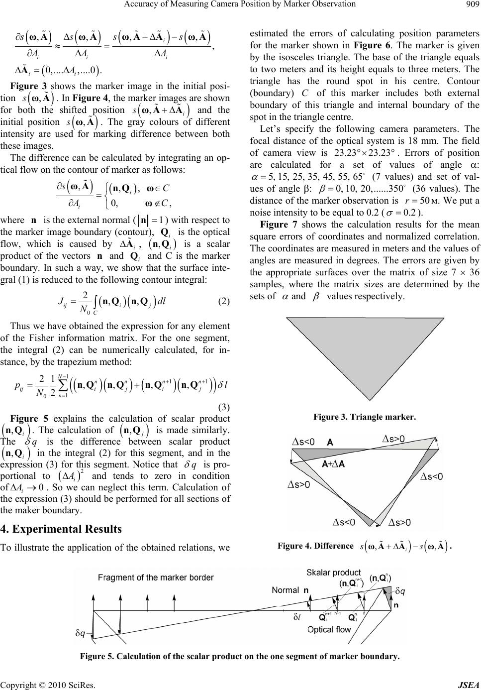


Accuracy of Measuring Camera Position by Marker Observation 909
 

 

,,, ,
0,....,....0 .
i
ii i
ii
sss s
AA A
A
 


 
ωAωAωAAωA
A


,




estimated the errors of calculating position parameters
for the marker shown in Figure 6. The marker is given
by the isosceles triangle. The base of the triangle equals
to two meters and its height equals to three meters. The
triangle has the round spot in his centre. Contour
(boundary) of this marker includes both external
boundary of this triangle and internal boundary of the
spot in the triangle centre.
C
Figure 3 shows the marker image in the initial posi-
tion . In Figure 4, the marker images are shown
for both the shifted position and the
initial position . The gray colours of different
intensity are used for marking difference between both
these images.

,sωA


,i sωAA


,sωA

Let’s specify the following camera parameters. The
focal distance of the optical system is 18 mm. The field
of camera view is . Errors of position
are calculated for a set of values of angle :
(7 values) and set of val-
ues of angle : (36 values). The
distance of the marker observation is м. We put a
noise intensity to be equal to 0.2 (
23.23 23.23
5, 55,65
0, 10,20,......350
5, 15,25,35,4  


r
0.2
50


).
The difference can be calculated by integrating an op-
tical flow on the contour of marker as follows:


,,,
0, ,
i
i
sC
AC




ωAnQ ω
ω

where is the external normal ( n1n) with respect to
the marker image boundary (contour), is the optical
flow, which is caused by
i
Q
i

A
, is a scalar
product of the vectors and i
Q and C is the marker
boundary. In such a way, we show that the surface inte-
gral (1) is reduced to the following contour integral:

,i nQ
Figure 7 shows the calculation results for the mean
square errors of coordinates and normalized correlation.
The coordinates are measured in meters and the values of
angles are measured in degrees. The errors are given by
the appropriate surfaces over the matrix of size 7  36
samples, where the matrix sizes are determined by the
sets of

and

values respectively.

n
 
0
2,,
iji j
C
J
dl
N
nQ nQ (2)
Thus we have obtained the expression for any element
of the Fisher information matrix. For the one segment,
the integral (2) can be numerically calculated, for in-
stance, by the trapezium method:
   
111
1
0
21 ,,, ,
2
Nnnn n
iji jij
n
pl
N




nQ nQnQnQ
(3)
Figure 3. Triangle marker.
Figure 5 explains the calculation of scalar product
. The calculation of

,i nQ



,
j
nQ is made similarly.
The q

is the difference between scalar product
in the integral (2) for this segment, and in the
expression (3) for this segment. Notice that

,i nQ

q

is pro-
portional to

2
i
A
 and tends to zero in condition
of . So we can neglect this term. Calculation of
the expression (3) should be performed for all sections of
the maker boundary.
0
i
A
4. Experimental Results
Figure 4. Difference .

,,
i
ss ωAAωA
 
 To illustrate the application of the obtained relations, we
Figure 5. Calculation of the scalar product on the one segment of marker boundary.

Accuracy of Measuring Camera Position by Marker Observation 910
Figure 6. Marker shape.
Accordingly to Figure 7, for the distance of 50 m and
the noise intensity 0.2

, the range r can be meas-
ured with error 0.02
r0.04


.05 0.4
m, as well as the dis-
placement in a CCD matrix plane can be measured with
errors VU , 0

  m. Rotation around the vec-
tor can be measured with the error .
As followed from Figure 7, the functional dependences
of measurement errors and normalized correlation of
linear and angular coordinates are very complicated
functions. We have considered the maker of uniform
brightness. In this case, only the contrast boundary oper-
ates in the marker image. The calculated precision values
are much higher than the similar values in [7] that are
based on using a small set of features (points of interest)
of the marker. Using the boundaries of marker image for
measurement provides an increase of the measurement
precision. Mention should be made that optical system
distortions and low resolution of CCD camera can seri-
ously deteriorate the precision of measurement. Joint
analysis of noise and camera resolution influence on the
precision of measurement is complicated enough.
r0.015 0.04

 

The above values of the mean square error and the
normalized correlation should be taken in an account in
creating the computer vision system. The significant
values of the normalized correlation show the consider-
able dependences between control loops of object posi-
tion coordinates. This fact should be taken into account
in the control system. The development of a computer
vision system should be carried out together with the
development of the marker shape.
α°
β°
σ
r
[m]
α°
β°
σ
v
[m]
α°
β°
σ
u
[m]
α°
β°
σ
γ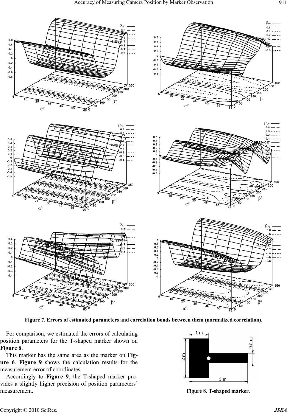
°

Accuracy of Measuring Camera Position by Marker Observation911
α°
β°
ρ
rv
α°
β°
ρru
α°
β°
ρ
rγ
α°
β°
ρ
uv
α°
β°
ρ
vγ
α°
β°
ρ
uγ
Figure 7. Errors of estimated parameters and correlation bonds between them (normalized correlation).
For comparison, we estimated the errors of calculating
position parameters for the T-shaped marker shown on
Figure 8.
This marker has the same area as the marker on Fig-
ure 6. Figure 9 shows the calculation results for the
measurement error of coordinates.
Accordingly to Figure 9, the T-shaped marker pro-
vides a slightly higher precision of position parameters’
measurement.
Figure 8. T-shed marker. ap

Accuracy of Measuring Camera Position by Marker Observation 912
[m]
α°
β°
σ
r
α°
β°
[m]
σ
v
α°
β°
[m]
σ
u
° σ
γ
α°
β°
Figure 9. Errors of estimated parameters for T-shaped marker.
5. Conclusions
The new method has been proposed for estimating the
errors of determining the TV camera position. This
method is based on using the marker image of a given
shape. The method allows us to estimate the measure-
ment errors depending on shooting conditions and CVS
parameters. The obtained error's estimations are useful
for development of CVSs and particularly for optimiza-
tion of their parameters.
6. Acknowledgement
This work was supported by the Russian Foundation for
Basic Research, project no. 09-01-00573-а.
REFERENCES
[1] C. De Wagter and J. A. Mulder, “Towards Vision-Based
UAV Situation Awareness,” Proceedings of the AIAA
Guidance, Navigation, and Control Conference, San
Francisco, California, August 2005, pp. AIAA-2005-
5872.
[2] S. Saripalli, J. F. Montgomery and G. S. Sukhatme,
“Visually-Guided Landing of an Unmanned Aerial Vehi-
cle,” IEEE Transactions on Robotics and Automation,
Vol. 19, No. 3, June 2003, pp. 371-380.
[3] S. Saripalli and G. S. Sukhatme, “Landing a Helicopter
on a Moving Target,” Proceedings of IEEE International
Conference on Robotics and Automation (ICRA’2007),
Roma, Italy, April 2007, pp. 2030-2035.
[4] T. Kubota, S. Sawai, T. Misu, T. Hashimoto, J. Kawagu-
chi and A. Fujiwara, “Autonomous Landing System for
MUSES-C Sample Return Mission,” Proceedings of the
Fifth International Symposium on Artificial Intelligence,
Robotics and Automation in Space (ISAIRAS’99), ESA
SP-440, Noordwijk, The Netherlands, June 1999, pp.
615-620.
[5] C. S. Sharp, O. Shakernia and S. S. Sastry, “A Vision
System for Landing an Unmanned Aerial Vehicle,” Pro-
ceedings of IEEE International Conference on Robotics
and Automation (ICRA 2001), Seoul, Korea, May 2001,

Accuracy of Measuring Camera Position by Marker Observation913
pp. 1720-1727.
[6] C. Akinli, “Semi-Autonomous Terminal Phase Spacecraft
Docking Attitude Determination and Control,” 2004.
http://cengiz.akinli.org/research/vsgc-2004.pdf
[7] V. A. Grishin, “Precision Estimation of Camera Position
Measurement Based on Docking Marker Observation,”
Pattern Recognition and Image Analysis, Vol. 20, No. 3,
2010, pp. 341-348.
[8] H. Cramer, “Mathematical Methods of Statistics,”
Princeton University Press, USA, 1946.
[9] I. A. Ibragimov and R. Z. Khasiminskii, “Asymptotic
Estimation Theory,” Nauka, Moscow, 1979.
[10] A. B. Kryanev and G. V. Lukin “Mathematical Methods
for Processing Indeterminate Data,” Fizmatlit, Moscow,
2003.
[11] H. L. Van Trees, “Detection, Estimation, and Modulation
Theory, Part 1: Detection, Estimation, and Linear Modu-
lation Theory,” John Wiley & Sons Inc., New York,
2001.