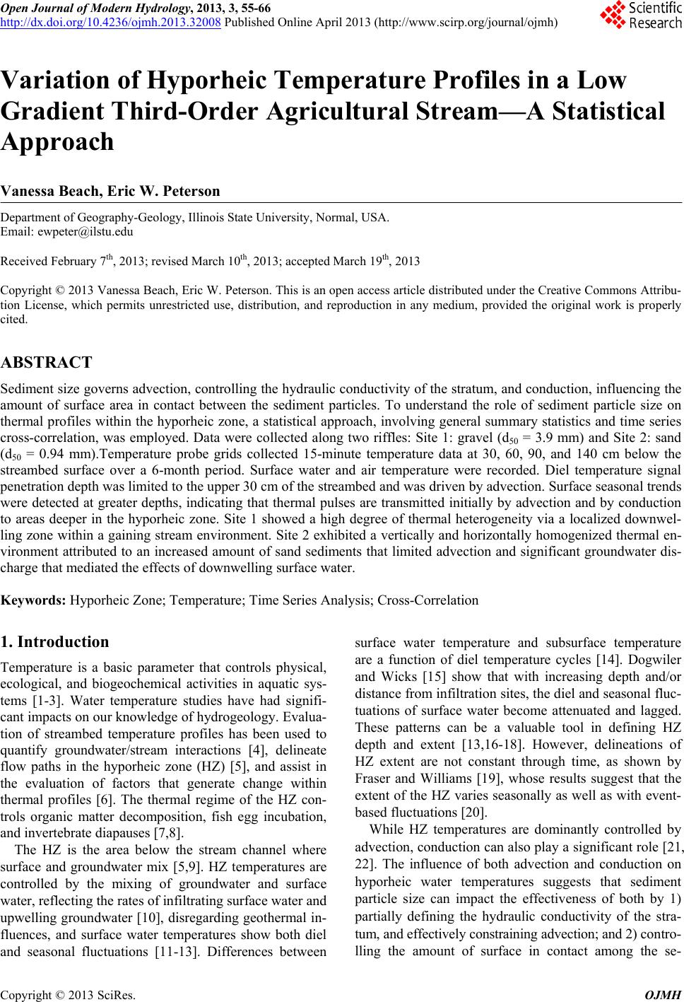
Open Journal of Modern Hydrology, 2013, 3, 55-66
http://dx.doi.org/10.4236/ojmh.2013.32008 Published Online April 2013 (http://www.scirp.org/journal/ojmh)
55
Variation of Hyporheic Temperature Profiles in a Low
Gradient Third-Order Agricultural Stream—A Statistical
Approach
Vanessa Beach, Eric W. Peterson
Department of Geography-Geology, Illinois State University, Normal, USA.
Received February 7th, 2013; revised March 10th, 2013; accepted March 19th, 2013
Copyright © 2013 Vanessa Beach, Eric W. Peterson. This is an open access article distributed under the Creative Commons Attribu-
tion License, which permits unrestricted use, distribution, and reproduction in any medium, provided the original work is properly
cited.
ABSTRACT
Sediment size governs advection, controlling the hydraulic conductivity of the stratum, and conduction, influencing the
amount of surface area in contact between the sediment particles. To understand the role of sediment particle size on
thermal profiles within the hyporheic zone, a statistical approach, involving general summary statistics and time series
cross-correlation, was employed. Data were collected along two riffles: Site 1: gravel (d50 = 3.9 mm) and Site 2: sand
(d50 = 0.94 mm).Temperature probe grids collected 15-minute temperature data at 30, 60, 90, and 140 cm below the
streambed surface over a 6-month period. Surface water and air temperature were recorded. Diel temperature signal
penetration depth was limited to the upper 30 cm of the streambed and was driven by advection. Surface seasonal trends
were detected at greater depths, indicating that thermal pulses are transmitted initially by advection and by conduction
to areas deeper in the hyporheic zone. Site 1 showed a high degree of thermal heterogeneity via a localized downwel-
ling zone within a gaining stream environment. Site 2 exhibited a vertically and horizontally homogenized thermal en-
vironment attributed to an increased amount of sand sediments that limited advection and significant groundwater dis-
charge that mediated the effects of downwelling surface water.
Keywords: Hyporheic Zone; Temperature; Time Series Analysis; Cross-Correlation
1. Introduction
Temperature is a basic parameter that controls physical,
ecological, and biogeochemical activities in aquatic sys-
tems [1-3]. Water temperature studies have had signifi-
cant impacts on our knowledge of hydrogeology. Evalua-
tion of streambed temperature profiles has been used to
quantify groundwater/stream interactions [4], delineate
flow paths in the hyporheic zone (HZ) [5], and assist in
the evaluation of factors that generate change within
thermal profiles [6]. The thermal regime of the HZ con-
trols organic matter decomposition, fish egg incubation,
and invertebrate diapauses [7,8].
The HZ is the area below the stream channel where
surface and groundwater mix [5,9]. HZ temperatures are
controlled by the mixing of groundwater and surface
water, reflecting the rates of infiltrating surface water and
upwelling groundwater [10], disregarding geothermal in-
fluences, and surface water temperatures show both diel
and seasonal fluctuations [11-13]. Differences between
surface water temperature and subsurface temperature
are a function of diel temperature cycles [14]. Dogwiler
and Wicks [15] show that with increasing depth and/or
distance from infiltration sites, the diel and seasonal fluc-
tuations of surface water become attenuated and lagged.
These patterns can be a valuable tool in defining HZ
depth and extent [13,16-18]. However, delineations of
HZ extent are not constant through time, as shown by
Fraser and Williams [19], whose results suggest that the
extent of the HZ varies seasonally as well as with event-
based fluctuations [20].
While HZ temperatures are dominantly controlled by
advection, conduction can also play a significant role [21,
22]. The influence of both advection and conduction on
hyporheic water temperatures suggests that sediment
particle size can impact the effectiveness of both by 1)
partially defining the hydraulic conductivity of the stra-
tum, and effectively constraining advection; and 2) contro-
lling the amount of surface in contact among the se-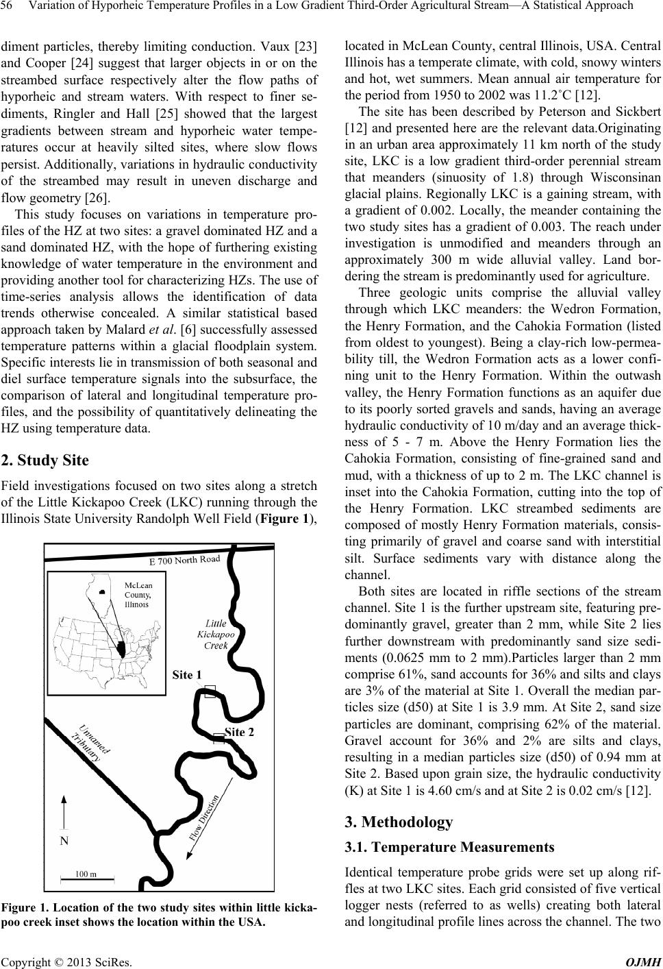

Variation of Hyporheic Temperature Profiles in a Low Gradient Third-Order Agricultural Stream—A Statistical Approach
56
diment particles, thereby limiting conduction. Vaux [23]
and Cooper [24] suggest that larger objects in or on the
streambed surface respectively alter the flow paths of
hyporheic and stream waters. With respect to finer se-
diments, Ringler and Hall [25] showed that the largest
gradients between stream and hyporheic water tempe-
ratures occur at heavily silted sites, where slow flows
persist. Additionally, variations in hydraulic conductivity
of the streambed may result in uneven discharge and
flow geometry [26].
This study focuses on variations in temperature pro-
files of the HZ at two sites: a gravel dominated HZ and a
sand dominated HZ, with the hope of furthering existing
knowledge of water temperature in the environment and
providing another tool for characterizing HZs. The use of
time-series analysis allows the identification of data
trends otherwise concealed. A similar statistical based
approach taken by Malard et al. [6] successfully assessed
temperature patterns within a glacial floodplain system.
Specific interests lie in transmission of both seasonal and
diel surface temperature signals into the subsurface, the
comparison of lateral and longitudinal temperature pro-
files, and the possibility of quantitatively delineating the
HZ using temperature data.
2. Study Site
Field investigations focused on two sites along a stretch
of the Little Kickapoo Creek (LKC) running through the
Illinois State University Randolph Well Field (Figure 1),
Figure 1. Location of the two study sites within little kicka-
poo creek inset shows the location within the USA.
located in McLean County, central Illinois, USA. Central
Illinois has a temperate climate, with cold, snowy winters
and hot, wet summers. Mean annual air temperature for
the period from 1950 to 2002 was 11.2˚C [12].
The site has been described by Peterson and Sickbert
[12] and presented here are the relevant data.Originating
in an urban area approximately 11 km north of the study
site, LKC is a low gradient third-order perennial stream
that meanders (sinuosity of 1.8) through Wisconsinan
glacial plains. Regionally LKC is a gaining stream, with
a gradient of 0.002. Locally, the meander containing the
two study sites has a gradient of 0.003. The reach under
investigation is unmodified and meanders through an
approximately 300 m wide alluvial valley. Land bor-
dering the stream is predominantly used for agriculture.
Three geologic units comprise the alluvial valley
through which LKC meanders: the Wedron Formation,
the Henry Formation, and the Cahokia Formation (listed
from oldest to youngest). Being a clay-rich low-permea-
bility till, the Wedron Formation acts as a lower confi-
ning unit to the Henry Formation. Within the outwash
valley, the Henry Formation functions as an aquifer due
to its poorly sorted gravels and sands, having an average
hydraulic conductivity of 10 m/day and an average thick-
ness of 5 - 7 m. Above the Henry Formation lies the
Cahokia Formation, consisting of fine-grained sand and
mud, with a thickness of up to 2 m. The LKC channel is
inset into the Cahokia Formation, cutting into the top of
the Henry Formation. LKC streambed sediments are
composed of mostly Henry Formation materials, consis-
ting primarily of gravel and coarse sand with interstitial
silt. Surface sediments vary with distance along the
channel.
Both sites are located in riffle sections of the stream
channel. Site 1 is the further upstream site, featuring pre-
dominantly gravel, greater than 2 mm, while Site 2 lies
further downstream with predominantly sand size sedi-
ments (0.0625 mm to 2 mm).Particles larger than 2 mm
comprise 61%, sand accounts for 36% and silts and clays
are 3% of the material at Site 1. Overall the median par-
ticles size (d50) at Site 1 is 3.9 mm. At Site 2, sand size
particles are dominant, comprising 62% of the material.
Gravel account for 36% and 2% are silts and clays,
resulting in a median particles size (d50) of 0.94 mm at
Site 2. Based upon grain size, the hydraulic conductivity
(K) at Site 1 is 4.60 cm/s and at Site 2 is 0.02 cm/s [12].
3. Methodology
3.1. Temperature Measurements
Identical temperature probe grids were set up along rif-
fles at two LKC sites. Each grid consisted of five vertical
logger nests (referred to as wells) creating both lateral
and longitudinal profile lines across the channel. The two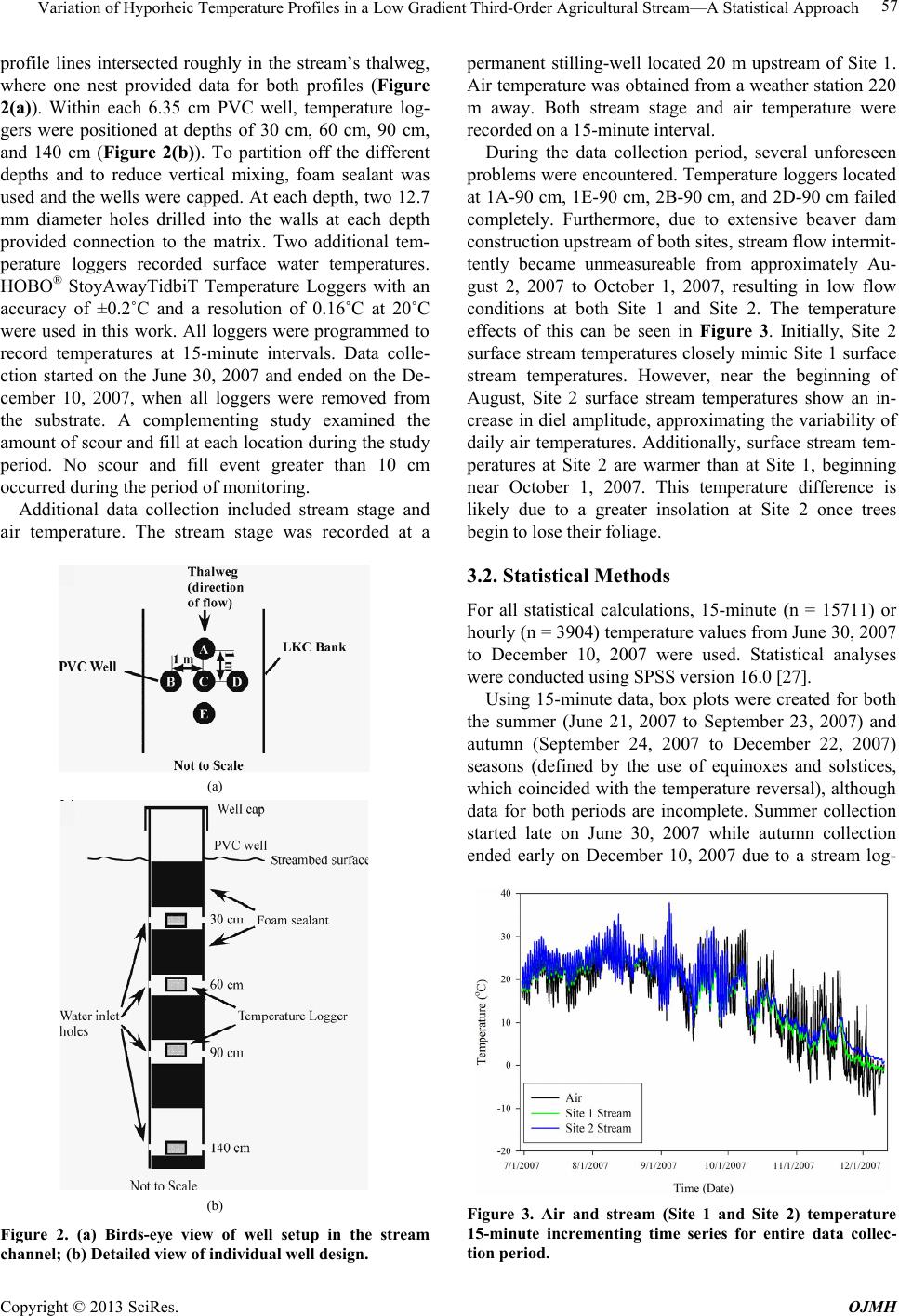

Variation of Hyporheic Temperature Profiles in a Low Gradient Third-Order Agricultural Stream—A Statistical Approach 57
profile lines intersected roughly in the stream’s thalweg,
where one nest provided data for both profiles (Figure
2(a)). Within each 6.35 cm PVC well, temperature log-
gers were positioned at depths of 30 cm, 60 cm, 90 cm,
and 140 cm (Figure 2(b)). To partition off the different
depths and to reduce vertical mixing, foam sealant was
used and the wells were capped. At each depth, two 12.7
mm diameter holes drilled into the walls at each depth
provided connection to the matrix. Two additional tem-
perature loggers recorded surface water temperatures.
HOBO® StoyAwayTidbiT Temperature Loggers with an
accuracy of ±0.2˚C and a resolution of 0.16˚C at 20˚C
were used in this work. All loggers were programmed to
record temperatures at 15-minute intervals. Data colle-
ction started on the June 30, 2007 and ended on the De-
cember 10, 2007, when all loggers were removed from
the substrate. A complementing study examined the
amount of scour and fill at each location during the study
period. No scour and fill event greater than 10 cm
occurred during the period of monitoring.
Additional data collection included stream stage and
air temperature. The stream stage was recorded at a
(a)
(b)
Figure 2. (a) Birds-eye view of well setup in the stream
channel; (b) Detailed view of individual well design.
permanent stilling-well located 20 m upstream of Site 1.
Air temperature was obtained from a weather station 220
m away. Both stream stage and air temperature were
recorded on a 15-minute interval.
During the data collection period, several unforeseen
problems were encountered. Temperature loggers located
at 1A-90 cm, 1E-90 cm, 2B-90 cm, and 2D-90 cm failed
completely. Furthermore, due to extensive beaver dam
construction upstream of both sites, stream flow intermit-
tently became unmeasureable from approximately Au-
gust 2, 2007 to October 1, 2007, resulting in low flow
conditions at both Site 1 and Site 2. The temperature
effects of this can be seen in Figure 3. Initially, Site 2
surface stream temperatures closely mimic Site 1 surface
stream temperatures. However, near the beginning of
August, Site 2 surface stream temperatures show an in-
crease in diel amplitude, approximating the variability of
daily air temperatures. Additionally, surface stream tem-
peratures at Site 2 are warmer than at Site 1, beginning
near October 1, 2007. This temperature difference is
likely due to a greater insolation at Site 2 once trees
begin to lose their foliage.
3.2. Statistical Methods
For all statistical calculations, 15-minute (n = 15711) or
hourly (n = 3904) temperature values from June 30, 2007
to December 10, 2007 were used. Statistical analyses
were conducted using SPSS version 16.0 [27].
Using 15-minute data, box plots were created for both
the summer (June 21, 2007 to September 23, 2007) and
autumn (September 24, 2007 to December 22, 2007)
seasons (defined by the use of equinoxes and solstices,
which coincided with the temperature reversal), although
data for both periods are incomplete. Summer collection
started late on June 30, 2007 while autumn collection
ended early on December 10, 2007 due to a stream log-
Figure 3. Air and stream (Site 1 and Site 2) temperature
15-minute incrementing time series for entire data collec-
tion period.

Variation of Hyporheic Temperature Profiles in a Low Gradient Third-Order Agricultural Stream—A Statistical Approach
58
ger failure. The temperature reversal (an isothermal pe-
riod during which air temperatures change from warm to
cool) occurring in early autumn, requires the separation
into seasons for unbiased summary statistics, and though
neither season is fully complete, the separation into sea-
sons gives a more illustrative overview of temperatures
than a grouped approach.
Time series cross-correlation, as described by Mangin
[20], was used to understand the relationships between
streambed temperatures within each site, as well as be-
tween sites in more detail.Time series cross-correlation
measures the relationship between two quantitative time
series, i.e. surface water temperature compared to hypor-
heic water temperature.The observations of two series
are correlated as various lags and leads, where the rela-
tionship is expressed by a cross-correlation coefficient (r)
equal to a value between −1 and 1, with values closest to
1 indicating the strongest relationship between the time
series.
The cross correlation coefficient (r) was obtained
using the formula proposed by Jenkins and Watts [28]
and as used by Malard et al. [6] to analyze streambed
time series temperature data:
,()
x
yk
k
x
y
C
rSS

With


1
,1
nk
iik
xyk i
Cn xxy







y (1)

,
x
yk
k
x
y
C
rSS

With


1
,1
nk
iik
xyk i
Cn yxy

x





 (2)
with x1, x2, …, xn = hourly values of surface water
temperature or temperatures, at shallower depths; y1,
y2, …, yn = hourly values of hyporheic water temperature
or temperatures at deeper depths; k = 0, 1, 2, …, m where
k is equal to the lag, and m is equal to the maximum
number of lags.
x
and
y
are means and Sx and Sy are
the means andthe standard deviations of the respective x
and y series.
For the evaluation of cross-correlation, the dataset was
reduced to hourly data to decrease the number of data
and to reduce the possibility of over-fitting the statistical
model. For the comparison of seasonal trends of both
surface water and hyporheic water temperatures a 24-
hour moving filter was applied to hourly data prior to
cross-correlation, removing diel temperature fluctuations.
Each filtered temperature at time t equaled the average
temperature from 12 hours prior to and 12 hours after
time t (including the temperature at time t in the ave-
raging).
For computation of between-site comparisons, gra-
dients (the difference between surface water tempera-
tures and temperatures at 140 cm depth) were used for
cross-correlation in substitution of actual recorded tem-
peratures. This eliminated the influence of differing sur-
face stream temperatures, and allowed instead a compa-
rison of the degree of temperature change with depth
between sites.
First-order differencing was applied to all time series
prior to cross-correlation, removing the data’s temporal
trend component and reducing autocorrelation. First-order
differencing is achieved by subtracting from each term of
the original series the preceding term.The transformation
generates a new series defined by: 1
ˆ()
ttt
XXX


where ˆt
X
= term of the filtered time series, and t
X
=
term of the original time series. All cross-correlations
were computed using a lag (k) of 1 hr, and a maximum
number of lags (m) of 125 determined so that mk

is
less than or equal to n/3 as recommended in the literature
[20].
For the evaluation of cross-correlation results, correla-
tion coefficients (r) equal to or greater than 0.2 were
treated as statistically significant. This was determined
based on the number of observations used, and assuming
rejection of the null hypothesis (there is no difference) if
a > 0.01.
4. Results
4.1. Summary Statistics
A distinct difference in temperature patterns is seen when
comparing summer and autumn results (Figure 4). In
summer, mean streambed temperatures fall at or below
mean surface stream temperatures, and pronounced coo-
ling is witnessed with depth into the streambed at both
sites. In autumn, these patterns are reversed with mean
surface stream temperatures at or below mean streambed
temperatures. A slight warming trend is also observed in
mean streambed temperatures with depth. Additionally,
temperatures appear more homogenized top to bottom,
where mean temperatures at increasing depths are not
distinctly different. It can be projected that the degree of
difference of autumn to summer temperature patterns
would increase in winter, and decrease again in spring
with the next reversal. Irrespective of the differences
observed between summer and autumn temperatures, a
decrease in temperature ranges with streambed depth is
experienced universally to varying degrees. In general,
the observations above show the data from this study to
be in line with general patterns witnessed in other HZ
temperature studies, such as by Dogwiler and Wicks [15],
in a karst environment featuring similar stream sediments
as at Site 1, and by White et al. [16] in a Michigan river.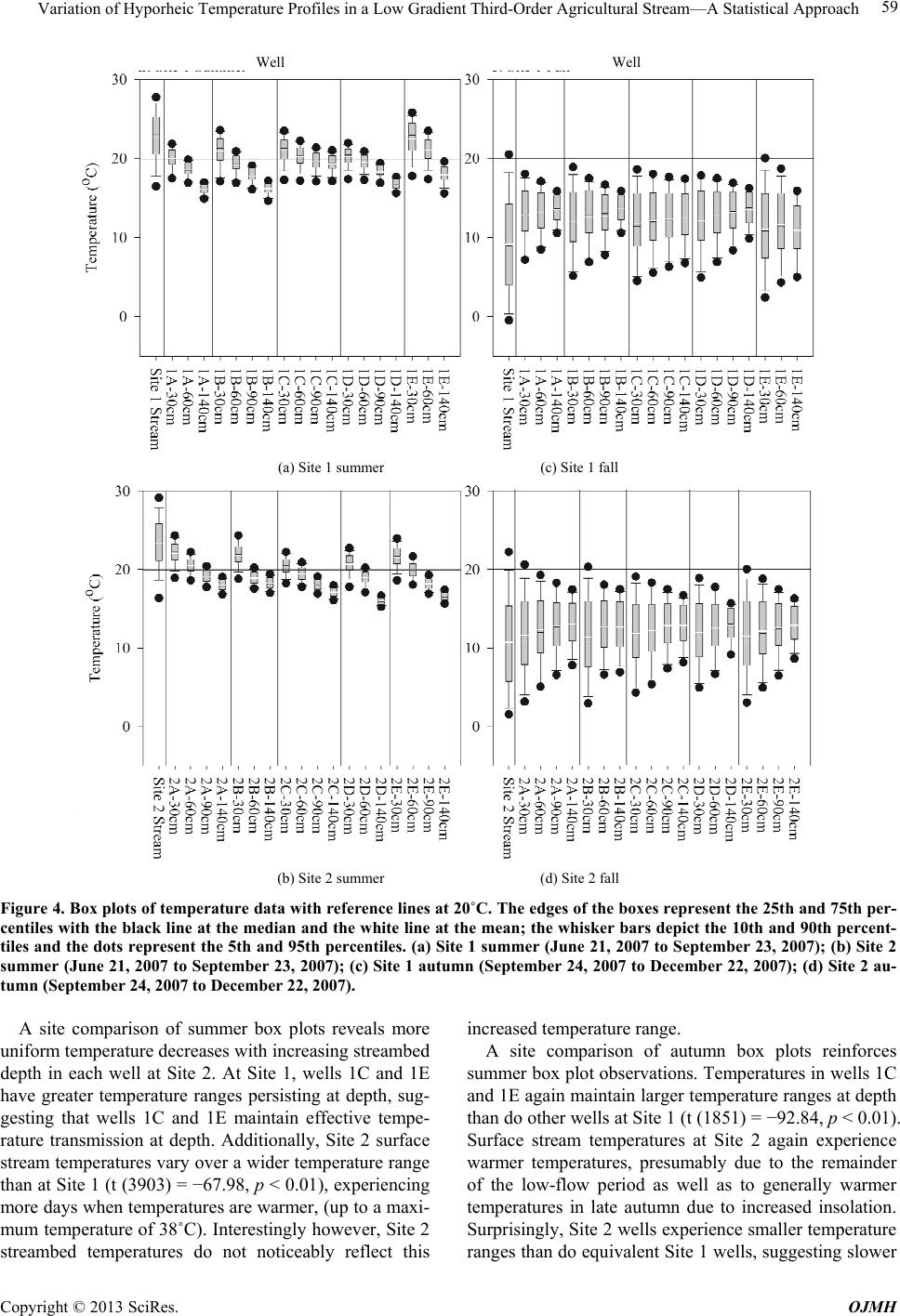

Variation of Hyporheic Temperature Profiles in a Low Gradient Third-Order Agricultural Stream—A Statistical Approach
59
Well Well
(a) Site 1 summer (c) Site 1 fall
(b) Site 2 summer (d) Site 2 fall
Figure 4. Box plots of temperature data with reference lines at 20˚C. The edges of the boxes represent the 25th and 75th per-
centiles with the black line at the median and the white line at the mean; the whisker bars depict the 10th and 90th percent-
tiles and the dots represent the 5th and 95th percentiles. (a) Site 1 summer (June 21, 2007 to September 23, 2007); (b) Site 2
summer (June 21, 2007 to September 23, 2007); (c) Site 1 autumn (September 24, 2007 to December 22, 2007); (d) Site 2 au-
tumn (September 24, 2007 to December 22, 2007).
A site comparison of summer box plots reveals more
uniform temperature decreases with increasing streambed
depth in each well at Site 2. At Site 1, wells 1C and 1E
have greater temperature ranges persisting at depth, sug-
gesting that wells 1C and 1E maintain effective tempe-
rature transmission at depth. Additionally, Site 2 surface
stream temperatures vary over a wider temperature range
than at Site 1 (t (3903) = −67.98, p < 0.01), experiencing
more days when temperatures are warmer, (up to a maxi-
mum temperature of 38˚C). Interestingly however, Site 2
streambed temperatures do not noticeably reflect this
increased temperature range.
A site comparison of autumn box plots reinforces
summer box plot observations. Temperatures in wells 1C
and 1E again maintain larger temperature ranges at depth
than do other wells at Site 1 (t (1851) = −92.84, p < 0.01).
Surface stream temperatures at Site 2 again experience
warmer temperatures, presumably due to the remainder
of the low-flow period as well as to generally warmer
temperatures in late autumn due to increased insolation.
Surprisingly, Site 2 wells experience smaller temperature
ranges than do equivalent Site 1 wells, suggesting slower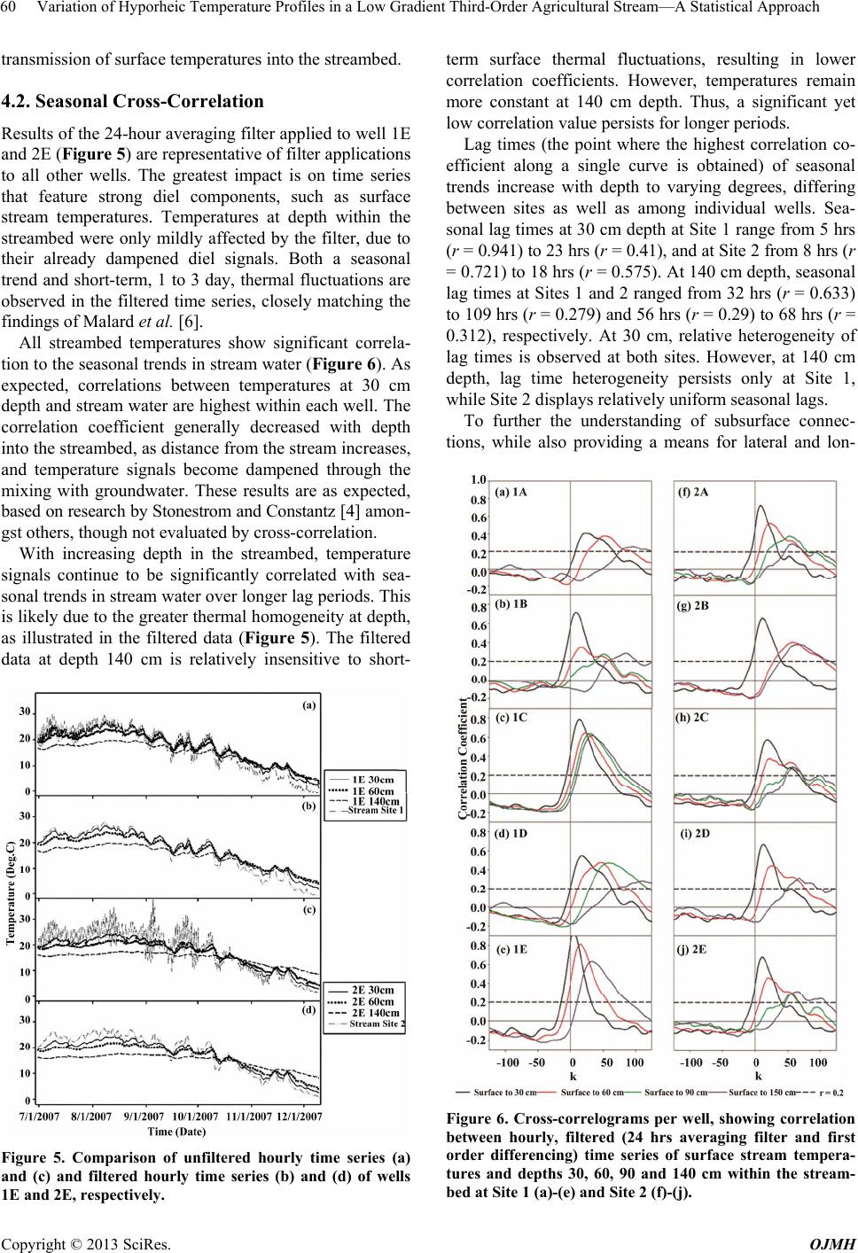

Variation of Hyporheic Temperature Profiles in a Low Gradient Third-Order Agricultural Stream—A Statistical Approach
60
transmission of surface temperatures into the streambed.
4.2. Seasonal Cross-Correlation
Results of the 24-hour averaging filter applied to well 1E
and 2E (Figure 5) are representative of filter applications
to all other wells. The greatest impact is on time series
that feature strong diel components, such as surface
stream temperatures. Temperatures at depth within the
streambed were only mildly affected by the filter, due to
their already dampened diel signals. Both a seasonal
trend and short-term, 1 to 3 day, thermal fluctuations are
observed in the filtered time series, closely matching the
findings of Malard et al. [6].
All streambed temperatures show significant correla-
tion to the seasonal trends in stream water (Figure 6). As
expected, correlations between temperatures at 30 cm
depth and stream water are highest within each well. The
correlation coefficient generally decreased with depth
into the streambed, as distance from the stream increases,
and temperature signals become dampened through the
mixing with groundwater. These results are as expected,
based on research by Stonestrom and Constantz [4] amon-
gst others, though not evaluated by cross-correlation.
With increasing depth in the streambed, temperature
signals continue to be significantly correlated with sea-
sonal trends in stream water over longer lag periods. This
is likely due to the greater thermal homogeneity at depth,
as illustrated in the filtered data (Figure 5). The filtered
data at depth 140 cm is relatively insensitive to short-
Figure 5. Comparison of unfiltered hourly time series (a)
and (c) and filtered hourly time series (b) and (d) of wells
1E and 2E, respectively.
term surface thermal fluctuations, resulting in lower
correlation coefficients. However, temperatures remain
more constant at 140 cm depth. Thus, a significant yet
low correlation value persists for longer periods.
Lag times (the point where the highest correlation co-
efficient along a single curve is obtained) of seasonal
trends increase with depth to varying degrees, differing
between sites as well as among individual wells. Sea-
sonal lag times at 30 cm depth at Site 1 range from 5 hrs
(r = 0.941) to 23 hrs (r = 0.41), and at Site 2 from 8 hrs (r
= 0.721) to 18 hrs (r = 0.575). At 140 cm depth, seasonal
lag times at Sites 1 and 2 ranged from 32 hrs (r = 0.633)
to 109 hrs (r = 0.279) and 56 hrs (r = 0.29) to 68 hrs (r =
0.312), respectively. At 30 cm, relative heterogeneity of
lag times is observed at both sites. However, at 140 cm
depth, lag time heterogeneity persists only at Site 1,
while Site 2 displays relatively uniform seasonal lags.
To further the understanding of subsurface connec-
tions, while also providing a means for lateral and lon-
Figure 6. Cross-correlograms per well, showing correlation
between hourly, filtered (24 hrs averaging filter and first
order differencing) time series of surface stream tempera-
tures and depths 30, 60, 90 and 140 cm within the stream-
bed at Site 1 (a)-(e) and Site 2 (f)-(j).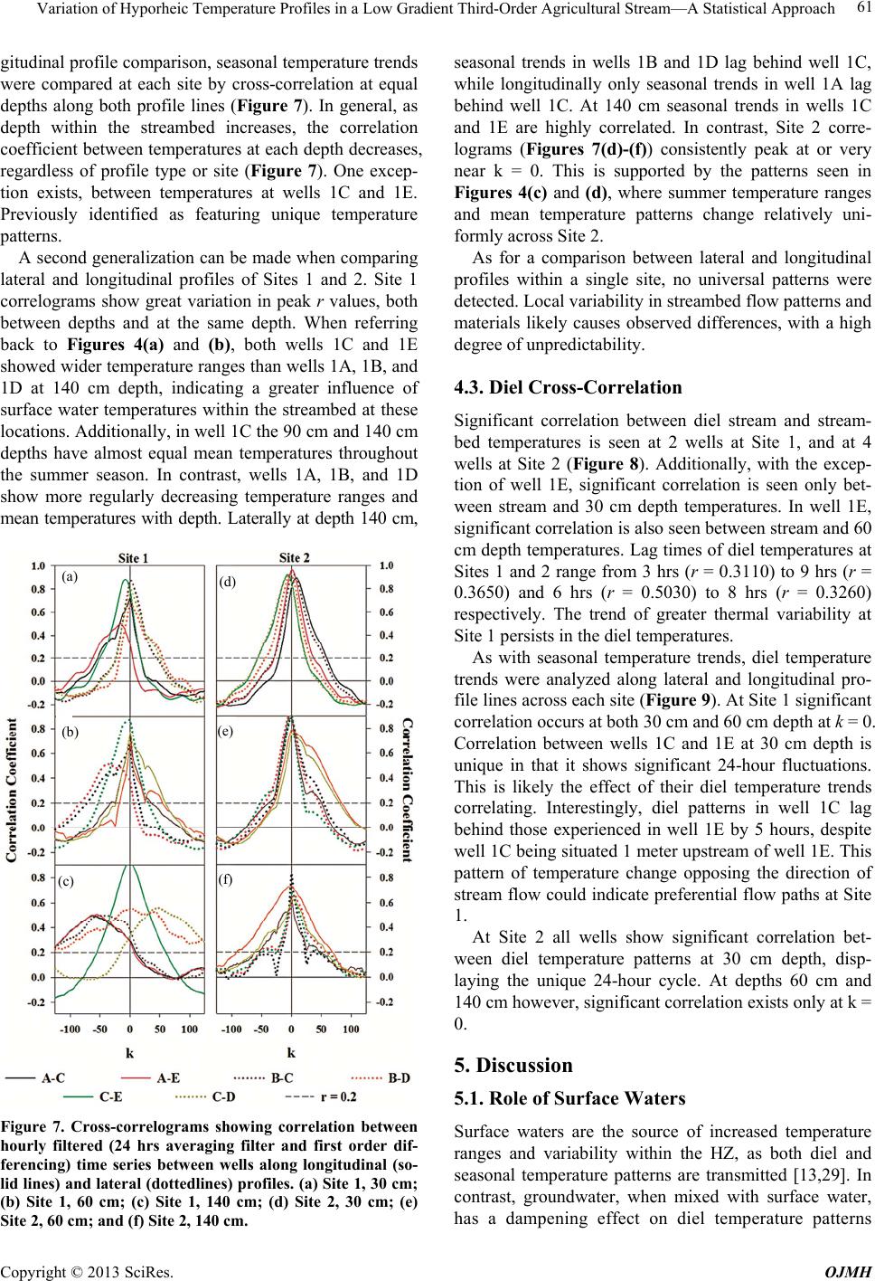

Variation of Hyporheic Temperature Profiles in a Low Gradient Third-Order Agricultural Stream—A Statistical Approach 61
gitudinal profile comparison, seasonal temperature trends
were compared at each site by cross-correlation at equal
depths along both profile lines (Figure 7). In general, as
depth within the streambed increases, the correlation
coefficient between temperatures at each depth decreases,
regardless of profile type or site (Figure 7). One excep-
tion exists, between temperatures at wells 1C and 1E.
Previously identified as featuring unique temperature
patterns.
A second generalization can be made when comparing
lateral and longitudinal profiles of Sites 1 and 2. Site 1
correlograms show great variation in peak r values, both
between depths and at the same depth. When referring
back to Figures 4(a) and (b), both wells 1C and 1E
showed wider temperature ranges than wells 1A, 1B, and
1D at 140 cm depth, indicating a greater influence of
surface water temperatures within the streambed at these
locations. Additionally, in well 1C the 90 cm and 140 cm
depths have almost equal mean temperatures throughout
the summer season. In contrast, wells 1A, 1B, and 1D
show more regularly decreasing temperature ranges and
mean temperatures with depth. Laterally at depth 140 cm,
(a)
(b)
(f)
(c)
(d)
(e)
Figure 7. Cross-correlograms showing correlation between
hourly filtered (24 hrs averaging filter and first order dif-
ferencing) time series between wells along longitudinal (so-
lid lines) and lateral (dottedlines) profiles. (a) Site 1, 30 cm;
(b) Site 1, 60 cm; (c) Site 1, 140 cm; (d) Site 2, 30 cm; (e)
Site 2, 60 cm; and (f) Site 2, 140 cm.
seasonal trends in wells 1B and 1D lag behind well 1C,
while longitudinally only seasonal trends in well 1A lag
behind well 1C. At 140 cm seasonal trends in wells 1C
and 1E are highly correlated. In contrast, Site 2 corre-
lograms (Figures 7(d)-(f)) consistently peak at or very
near k = 0. This is supported by the patterns seen in
Figures 4(c) and (d), where summer temperature ranges
and mean temperature patterns change relatively uni-
formly across Site 2.
As for a comparison between lateral and longitudinal
profiles within a single site, no universal patterns were
detected. Local variability in streambed flow patterns and
materials likely causes observed differences, with a high
degree of unpredictability.
4.3. Diel Cross-Correlation
Significant correlation between diel stream and stream-
bed temperatures is seen at 2 wells at Site 1, and at 4
wells at Site 2 (Figure 8). Additionally, with the excep-
tion of well 1E, significant correlation is seen only bet-
ween stream and 30 cm depth temperatures. In well 1E,
significant correlation is also seen between stream and 60
cm depth temperatures. Lag times of diel temperatures at
Sites 1 and 2 range from 3 hrs (r = 0.3110) to 9 hrs (r =
0.3650) and 6 hrs (r = 0.5030) to 8 hrs (r = 0.3260)
respectively. The trend of greater thermal variability at
Site 1 persists in the diel temperatures.
As with seasonal temperature trends, diel temperature
trends were analyzed along lateral and longitudinal pro-
file lines across each site (Figure 9). At Site 1 significant
correlation occurs at both 30 cm and 60 cm depth at k = 0.
Correlation between wells 1C and 1E at 30 cm depth is
unique in that it shows significant 24-hour fluctuations.
This is likely the effect of their diel temperature trends
correlating. Interestingly, diel patterns in well 1C lag
behind those experienced in well 1E by 5 hours, despite
well 1C being situated 1 meter upstream of well 1E. This
pattern of temperature change opposing the direction of
stream flow could indicate preferential flow paths at Site
1.
At Site 2 all wells show significant correlation bet-
ween diel temperature patterns at 30 cm depth, disp-
laying the unique 24-hour cycle. At depths 60 cm and
140 cm however, significant correlation exists only at k =
0.
5. Discussion
5.1. Role of Surface Waters
Surface waters are the source of increased temperature
ranges and variability within the HZ, as both diel and
seasonal temperature patterns are transmitted [13,29]. In
contrast, groundwater, when mixed with surface water,
has a dampening effect on diel temperature patterns

Variation of Hyporheic Temperature Profiles in a Low Gradient Third-Order Agricultural Stream—A Statistical Approach
62
Figure 8. Cross-correlograms per well (indicated by letters A through E), showing correlation between hourly transformed
(first order differencing) time series of surface stream temperatures and depths 30, 60, 90 and 140 cm within the streambed
t Site 1 (a)-(e) and Site 2 (a)-(e). a

Variation of Hyporheic Temperature Profiles in a Low Gradient Third-Order Agricultural Stream—A Statistical Approach 63
Figure 9. Cross-correlograms at 30 cm (a) and (d), 60 cm (b)
and (e), and 140 cm (c) and (e), showing correlation be-
tween hourly transformed (first order differencing) time
series between wells along longitudinal (solid lines) and
lateral (dotted lines) profiles at Site 1 and Site 2, respec-
tively.
within the HZ, as it imparts only seasonal temperature
trends [4,13]. The decreasing temperature ranges and
mean temperatures, as seen in box plots (Figure 4), can
be attributed to the mixing of surface and groundwater
and the increasing influence of groundwater with depth.
5.2. Differences between Site 1 & Site 2
Box plots reveal that while the stream water at Site 2
experienced greater temperature extremes than at Site 1,
the extremes were not observed in the streambed tem-
peratures at Site 2. This suggests that hyporheic ex-
change is lower at Site 2 than at Site 1. Possible ex-
planations include the allowance of less surface water
infiltration, the presence of increased groundwater dis-
charge, the presence of meander flow-through, or per-
haps the retardation of infiltration velocities associated
with the finer grain sizes of the substrate at Site 2 as
suggested by Ringler and Hall [25]. The hypothesis of
less surface water infiltration is tied to the discharge of a
greater groundwater component, dampening diel surface
water signals. This possible explanation is consistent
with the establishment of Site 2 as a gaining reach. The
second possibility of retarded infiltration velocities is
supported by Ringer and Hall [25], who found larger
temperature gradients between stream and hyporheic
waters at heavily silted sites, due to slower inter-gravel
flows. Based on grain size analyses, we believe that
while silt size particles are not prevalent at Site 2, the
small particles sizes and lower hydraulic conductivity, as
compared to Site 1, may exert a similar effect. Though
dampened in amplitude, diel surface water signals are
still transmitted down to a 30 cm depth almost univer-
sally across Site 2 (Figure 9).
In addition to increased dampening of surface thermal
trends, greater uniformity in thermal trends is seen in box
plot and cross-correlation results at Site 2. Thus, Site 2
has more uniform HZ flow path patterns associated with
more homogeneous sediment distribution. Vaux [23] and
Cooper [24] observed that larger objects in or on the
streambed surface respectively, cause significant disrup-
tions to HZ flow paths and thereby thermal patterns as
well, which does not appear to be the case at Site 2. Site
1 however, displays distinct thermal heterogeneity when
comparing thermal trends in wells 1A, 1B, and 1D, to
those in wells 1C and 1E, making the presence of sedi-
ment variations a possibility.While no large particles
were observed on the streambed surface, Buyck [30]
documented the presence of till anomalies in the stream
bed up to depths of 60 cm.
Numerical modeling of the area indicated that Site 1 is
a downwelling zone, while Site 2 is an upwelling zone
[31]. While the site-specific details are not addressed,
these flow dynamics potentially explain many of the
trends observed in the statistical results of this study, as
outlined below.Advection, as involved in a losing reach
or downwelling zone, is commonly considered the most
effective means of thermal transport, as fluid movement
is typically faster and more efficient at heat transmission
than the process of conduction. Therefore, the effective
transmission of diel temperature signals into the substrate
is likely due to advection of stream water into the HZ.
This goes hand-in-hand with the established tempera-
ture-based method of defining losing and gaining reaches
of a stream, where the presence of increased diel signal
transmission into the HZ is an indication of a losing
reach [4].
Lags between unfiltered hourly temperatures of the
stream and at 30 cm depth (showing diel temperature
variations) ranged from 3 to 9 hours. The smallest lag of
3 hours was experienced at Site 1, where sediments are
coarser and feature a higher hydraulic conductivity. Site
2, with a lower hydraulic conductivity, experienced lags
of 6 to 8 hours.
The persistent penetrations of diel surface water tem-
perature patterns to depths of 30 cm in wells 1C and 1E,
and to a depth of 60 cm (Figure 8) in well 1E, suggest
the influence of a strong vertical advective component at
Site 1. Additionally, these trends reinforce the identifi-
cation of Site 1 as a downwelling zone, and pinpoint
wells 1C and 1E as the point of most focused down-

Variation of Hyporheic Temperature Profiles in a Low Gradient Third-Order Agricultural Stream—A Statistical Approach
64
welling of surface water to a minimum depth of 30 cm in
both wells, and to a minimum depth of 60 cm in well 1E.
This is further reinforced by seasonal correlation coef-
ficients of surface water to 140 cm depth remaining
above 0.6 at both wells 1C and 1E, suggesting that sur-
face water seasonal variations are responsible for 60% of
the seasonal variability witnessed at this depth. It is
therefore likely that advection penetrates deeper than the
minimum values stated above, yet based on the available
data no conclusive statement can be made.
Though both wells 1C and 1E appear to be the location
of deepest surface water penetration, well 1E is the
location of fastest surface water penetration to a depth of
30 cm, as shown by correlation results between 30 cm
temperatures in wells 1C and 1E. Flow paths within the
HZ and streambed can be controlled by a large number
of factors. However, from what is known of Site 1 re-
garding sediment particle size and thermal heterogeneity,
it is very likely that both flow paths and thermal regimes
are impacted by sediment heterogeneities in the HZ and
streambed. Buyck [30] found gray clay in the streambed,
originating possibly from collapsed cut banks, or from
underlying till layers. Such clay in the HZ would act as
barriers to advection, and increase the chance of prefe-
rential flow path development, which could in turn lead
to uncharacteristic flow patterns, as supported by re-
search conducted by Vaux [23] and Becker et al. [26].
Site 2 flow path delineation is somewhat less precise
than at Site 1. The comparison of lateral and longitudinal
profiles at 30 cm depth reveals that the strongest corre-
lation exists in the longitudinal direction, following the
direction of stream flow. However, correlation between
lateral temperature patterns at 30 cm depth exists also.
This correlation reflects similar degrees of surface diel
signal penetration to 30 cm depth. At depths greater than
30 cm, correlation of diel patterns is only significant at k
= 0, suggesting lateral homogeneity of temperatures
across the site. Based on statistical results, we believe
flow paths at Site 2 are mostly in the longitudinal dire-
ction, at low velocities, and active surface water infiltra-
tion is limited to the upper 30 cm of the streambed. The
influence of lateral flow is supported by the numerical
modeling of Van der Hoven [31] showing the area to be
an outlet for flow from underneath a meander lobe.
5.3. Controls on Thermal Transport
The process of conduction, while in part dependent on
the thermal properties of a medium, is driven by tem-
perature gradients, where steeper temperature gradients
increase the effectiveness of conduction. Steepest tempe-
rature gradients appear to exist laterally at Site 1, bet-
ween vertically down-welling warmer temperatures in
well 1C and 1E, and cooler temperatures in wells 1A, 1B,
and 1D. Subsequently, conduction may be an important
mode of heat transport in the lateral direction at Site 1.
At Site 2 thermal gradients appear more gradual, sug-
gesting conduction will be kept to a minimum. However,
during the low-flow period at Site 2, the heating of
streambed sediments by solar radiation may have pro-
vided a steep thermal gradient, allowing conduction an
active role in the transport of heat into the HZ. A similar
proposition was put forward by Shepherd et al. [32].
However, there are situations where advection and ver-
tical conduction are of similar magnitude [22].
Quantitative delineation of the HZ based on thermal
trends has not been possible. Though statements can be
made as to where the HZ definitely persists, such as at 30
cm depth in the locations of wells 1C, 1E, 2A, 2B, 2D,
and 2E, where significant correlation to surface stream
diel temperature patterns was found, the exact cut-off
point between the HZ and groundwater environments is
difficult to pinpoint quantitatively without a thermal
groundwater signature for the study location.
It is also possible that the maximum logger installation
depth managed for this study was not deep enough to
penetrate beyond the HZ. Even at 140 cm depth, seasonal
temperature trends vary more than by the expected ±3˚C
[10] range from the annual mean air temperature of
11.2˚C. A likely alternative explanation to lacking pe-
netration depth is the impact of conduction on tempera-
tures at depth [22]. While the presence of advecting sur-
face water defines the extent of the HZ, the presence of
conduction may alter temperatures beyond the extent of
the HZ, effectively masking the true groundwater ther-
mal signature. Seasonal cross-correlation results between
surface water and 140 cm depth at both sites (Figure 6)
suggest at least 20% of the variability witnessed can still
be explained by surface water variability. This may be
coincidence, based on the large number of observations
used in the correlation, as well as the small degree of
change in the temperatures and the fact that groundwater
also has a seasonal signal. However, if not coincidence, it
seems possible that conduction could transmit 20% of the
surface thermal signature to a depth of 140 cm below the
streambed [22], especially considering that the seasonal
trends are transmitted into the upper 30 cm by advection,
leaving approximately 110 cm distance to be spanned by
conduction.
6. Conclusions
Stream-groundwater interaction and HZ sediment phy-
sical and thermal properties are the major determining
factors for temperature patterns within the HZ, simu-
ltaneously defining HZ flow paths of surface and ground-
water, and the effectiveness of temperature transmission
into the subsurface. Consequently, differences in one or
all of these properties must exist between Sites 1 and 2 to
explain the differences in temperature behavior, for al-

Variation of Hyporheic Temperature Profiles in a Low Gradient Third-Order Agricultural Stream—A Statistical Approach 65
though both site comparisons (Figures 7 and 8) show
little difference between thermal gradients, local diffe-
rences were observed in all other statistical results.
Overall, distinct differences were identified in the ther-
mal profiles of Sites 1 and 2. Site 1 appears as a down-
welling zone with surface water penetrating deepest into
the HZ at the location of wells 1C and 1E. Site 2 was
characterized as a gaining reach, where the balancing
between down-welling surface water and upwelling
groundwater temperatures resulted in a more homo-
genized thermal environment. Additionally, a dampening
of diel surface stream temperature ranges was noticed in
upper HZ temperatures at Site 2. This dampening was
attributed to a variety of possible causes, including a
significant discharging groundwater component, which
would produce a dampening effect on diel temperatures
as previously outlined. This explanation is in line with
Site 2 being recognized as a gaining reach. Additionally,
the possibility of an increased percentage of finer sedi-
ments at the site was considered, resulting in slightly
retarded inter-gravel flows causing dampening associated
with the longer thermal transmission times.
A correlation between increased sediment homoge-
neity and more homogeneous thermal profiles was noted,
though the lack of multiple sites makes definitive inter-
pretation difficult. However, it has been established in
the literature that larger sediment particles as well as po-
ssible low permeability zones can disrupt HZ flow paths
and thermal regimes by altering the flowpaths[23,26].
The transmission of diel signals is limited by the
efficiency of advection and diel thermal transfer requires
higher transmission speeds than seasonal temperature
signals. Supporting this, the deepest penetration depth of
diel temperature patterns was 60 cm in well 1E, while
seasonal surface temperature patterns were detected uni-
versally to a depth of 140 cm.
Thermal differences in lateral and longitudinal profiles
were detected, and were attributed to variations in factors
affecting thermal transport, such as the presence of prefe-
rential flow paths. The longitudinal profile exhibited a
greater tendency for progressive transmission of thermal
signals in the downstream direction, though a thermal
transmission against the direction of stream flow was
detected at Site 1.
Finally, only qualitative delineation of the HZ was
possible in this study.The main limitation was the lack of
a specific thermal groundwater signature for the study
area. The persistence of surface seasonal temperature
trends beyond the extent of surface diel temperature is
likely due to the influence of conduction on temperatures
below the reach of advection [33,34].
Both sediment particle size and degree of sorting
impact thermal profiles. Site 1 (poorly sorted gravels)
showed a high degree of thermal heterogeneity through
preferential flow paths (local downwelling zone). Site 2
(moderately sorted sands) showed a vertically and late-
rally homogenized thermal environment with no defined
preferential flow paths. Meander flow-through discharge
can have a significant impact on streambed temperatures.
The transmission of diel signals is limited by the effi-
ciency of advection, requiring higher transmission speeds
than seasonal temperature signals. The deepest pene-
tration depth of diel temperature patterns was 60 cm in
well 1E, where a local downwelling zone exists. Surface
water temperatures influence the thermal regime not only
of the hyporheic ecotone, but also of the shallow ground-
water environment. Seasonal surface temperature patterns
were detected universally to a depth of 140 cm.
7. Acknowledgements
The authors would like to extend a sincere thank to the
following organizations: The Bloomington Normal Wa-
stewater Reclamation District for access to the study site.
The Geological Society of America (student research
grant-Beach), Grant-In-Aid of Research from Sigma Xi
(student research grant-Beach), and the PADI Foundation,
for funding of this study.
REFERENCES
[1] H. B. N. Hynes, “Ecology of Running Waters,” Liverpool
University Press, Liverpool, 1970.
[2] G. C. Poole and C. H. Berman, “An Ecological Perspec-
tive on In-Stream Temperature: Natural Heat Dynamics
and Mechanisms of Human-CausedThermal Degrada-
tion,” Environmental Management, Vol. 27, No. 6, 2001,
pp. 787-802. doi:10.1007/s002670010188
[3] J. V. Ward, “THERMAL Characteristics of Running Wa-
ters,” Hydrobiologia, Vol. 125, No. 1, 1985, pp. 31-46.
doi:10.1007/BF00045924
[4] D. A. Stonestrom and J. Constantz, “Heat as a Tool for
Studying the Movement of Ground Water Near Streams,”
US Geological Survey, Denver, 2003.
[5] B. Conant, “Delineating and Quantifying Ground Water
Discharge Zones Using Streambed Temperatures,” Ground
Water, Vol. 42, No. 2, 2004, pp. 243-257.
doi:10.1111/j.1745-6584.2004.tb02671.x
[6] F. Malard, A. Mangin, U. Uehlinger and J. V. Ward,
“Thermal Heterogeneity in the Hyporheic Zone of a Gla-
cial Floodplain,” Canadian Journal of Fisheries and Aqua-
tic Sciences, Vol. 58, No. 7, 2001, pp. 1319-1335.
doi:10.1139/f01-079
[7] M. Hondzo and H. G. Stefan, “Riverbed Heat Conduction
Prediction,” Water Resources Research, Vol. 30, No. 5,
1994, pp. 1503-1513. doi:10.1029/93WR03508
[8] S. E. Silliman, J. Ramirez and R. L. McCabe, “Quantif-
ing Downflow through Creek Sediments Using Tempera-
ture Time Series: One-Dimensional Solution Incorporat-
ing Measured Surface Temperature,” Journal of Hydrol-
ogy, Vol. 167, No. 1-4, 1995, pp. 99-119.

Variation of Hyporheic Temperature Profiles in a Low Gradient Third-Order Agricultural Stream—A Statistical Approach
66
doi:10.1016/0022-1694(94)02613-G
[9] M. Hayashi and D. O. Rosenberry, “Effects of Ground
Water Exchange on the Hydrology and Ecology of Sur-
face Water,” Ground Water, Vol. 40, No. 3, 2002, pp.
309-316. doi:10.1111/j.1745-6584.2002.tb02659.x
[10] D. Deming, “Introduction to Hydrogeology,” McGraw
Hill, Boston, 2002.
[11] M. P. Anderson, “Heat as a Ground Water Tracer,” Ground
Water, Vol. 43, No. 6, 2005, pp. 951-968.
doi:10.1111/j.1745-6584.2005.00052.x
[12] E. W. Peterson and T. B. Sickbert, “Stream Water Bypass
through a Meander Neck, Laterally Extending the Hy-
porheic Zone,” Hydrogeology Journal, Vol. 14, No. 8,
2006, pp. 1443-1451. doi:10.1007/s10040-006-0050-3
[13] C. Schmidt, M. Bayer-Raich and M. Schirmer, “Characte-
rization of Spatial Heterogeneity of Groundwater-Stream
Water Interactions Using Multiple Depth Streambed Tem-
perature Measurements at the Reach Scale,” Hydrology
and Earth System Sciences Earth System Sciences Dis-
cussions, Vol. 3, 2006, pp. 1419-1446.
doi:10.5194/hessd-3-1419-2006
[14] A. S. Arrigoni, et al., “Buffered, Lagged, or Cooled? Dis-
entangling Hyporheic Influences on Temperature Cycles
in Stream Channels,” Water Resources Research, Vol. 44,
No. 9, 2008, Article ID: W09418.
doi:10.1029/2007WR006480
[15] T. J. Dogwiler and C. M. Wicks, “Thermal Variations in
the Hyporheic Zone of a Karst Stream,” Speleogenesis
and Evolution of Karst Aquifers, Vol. 3, No. 1, 2005, pp.
1-11.
[16] D. S. White, C. Elzinga, H. and S. P. Hendricks, “Tem-
perature Patterns within the Hyporheic Zone of a North-
ern Michigan River,” Journal of North American Bentho-
logical Society, Vol. 6, No. 2, 1987, pp. 85-91.
doi:10.2307/1467218
[17] C. E. Hatch, A. T. Fisher, J. S. Revenaugh, J. Constantz
and C. Ruehl, “Quantifying Surface Water-Groundwater
Interactions Using Time Series Analysis of Streambed
Thermal Records: Method Development,” Water Resour-
ces Research, Vol. 42, No. 10, 2006, Article ID: W10410.
[18] C. Schmidt, B. Conant Jr., M. Bayer-Raich and M. Schir-
mer, “Evaluation and Field-Scale Application of a Simple
Analytical Method to Quantify Groundwater Discharge
Using Mapped Streambed Temperatures,” Journal of Hy-
drology, 2007.
[19] B. G. Fraser and D. D. Williams, “Seasonal Boundary
Dynamics of a Groundwater/Surface-Water Ecotone,” Eco-
logy, Vol. 79, No. 6, 1998, pp. 2019-2031.
[20] A. Mangin, “For a Better Knowledge of Hydrological
Systems from Correlogram and Variance Spectral Den-
sity,” Journal of Hydrology, Vol. 67, No. 1-4, 1984, pp.
25-43. doi:10.1016/0022-1694(84)90230-0
[21] E. C. Evans, M. T. Greenwood and G. E. Petts, “Thermal
Profiles within River Beds,” Hydrological Processes, Vol.
9, No. 1, 1995, pp. 19-25. doi:10.1002/hyp.3360090103
[22] E. T. Hester, M. W. Doyle and G. C. Poole, “The Influ-
ence of In-Stream Structures on Summer Water Tem-
peratures via Induced Hyporheic Exchange,” Limnology
and Oceanography, Vol. 54, No. 1, 2009, pp. 355-367.
doi:10.4319/lo.2009.54.1.0355
[23] W. G. Vaux, “Intergravel Flow and Interchange of Water
in a Streambed,” Fishery Bulletin, Vol. 66, No. 3, 1968,
pp. 479-489.
[24] A. C. Cooper, “The Effect of Transported Stream Sedi-
ments on the Survival of Sockeye and Pink Salmon Eggs
and Alevins,” International Pacific Salmon Fishery Com-
mission Bulletin, Vol. 18, 1965, p. 75.
[25] N. H. Ringler and J. D. Hall, “Effects of Logging on Tem-
perature, and Dissolved Oxygen in Spawning Beds,” Trans-
actions of the American Fisheries Society, Vol. 104, No.
1, 1975, pp. 111-121.
doi:10.1577/1548-8659(1975)104<111:EOLOWT>2.0.C
O;2
[26] M. W. Becker, T. Georgianb, H. Ambrosea, J. Siniscal-
chia and K. Fredricka, “Estimating Flow and Flux of
Ground Water Discharge Using Water Temperature and
Velocity,” Journal of Hydrology, Vol. 296, No. 1-4, 2004,
pp. 221-233. doi:10.1016/j.jhydrol.2004.03.025
[27] “SPSS for Windows Rel. 16.0.1.,” SPSS Inc., Chicago,
2007.
[28] G. M. Jenkins and D. G. Watts, “Spectral Analysis and Its
Applications,” Holden-Day, San Francisco, 1968.
[29] M. Brunke and T. Gonser, “The Ecological Significance
of Exchange Processes between Rivers and Groundwater
(Special Review),” Freshwater Biology, Vol. 37, No. 1,
1997, pp. 1-33. doi:10.1046/j.1365-2427.1997.00143.x
[30] M. S. Buyck, “Tracking Nitrate Loss and Modeling Flow
through the Hyporheic Zone of a Low Gradient Stream
through the Use of Conservative Tracers,” Illinois State
University, Normal, 2005.
[31] S. van der Hoven, N. Fromm and E. Peterson, “Quantif-
ing Nitrogen Cycling Beneath a Meander of a Low Gra-
dient, N-Impacted, Agricultural Stream Using Tracers and
Numerical Modelling,” Hydrological Processes, Vol. 22,
No. 8, 2008, pp. 1206-1215.
[32] B. G. Shepherd, G. F. Hartman and W. J. Wilson, “Rela-
tionships between Stream and Intragravel Temperatures
in Coastal Drainages and Some Implications for Fisheries
Workers,” Canadian Journal of Fisheries and Aquatic
Sciences, Vol. 43, No. 9, 1986, pp. 1818-1822.
doi:10.1139/f86-226
[33] E. Hoehn and O. A. Cirpka, “Assessing Hyporheic Zone
Dynamics in Two Alluvial Flood Plains of the Southern
Alps Using Water Temperature and Tracers,” Hydrology
and Earth System Sciences Discussions, Vol. 3, No. 2,
2006, pp. 335-364. doi:10.5194/hessd-3-335-2006
[34] W. W. Lapham, “Use of Temperature Profiles Beneath
Streams to Determine Rates of Vertical Ground-Water
Flow and Vertical Hydraulic Conductivity,” United States
Geological Survey, Reston, 1989, p. 35.