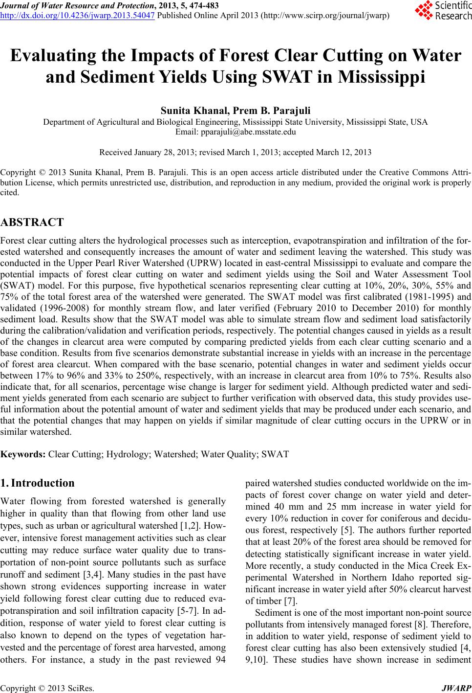
 Journal of Water Resource and Protection, 2013, 5, 474-483 http://dx.doi.org/10.4236/jwarp.2013.54047 Published Online April 2013 (http://www.scirp.org/journal/jwarp) Evaluating the Impacts of Forest Clear Cutting on Water and Sediment Yields Using SWAT in Mississippi Sunita Khanal, Prem B. Parajuli Department of Agricultural and Biological Engineering, Mississippi State University, Mississippi State, USA Email: pparajuli@abe.msstate.edu Received January 28, 2013; revised March 1, 2013; accepted March 12, 2013 Copyright © 2013 Sunita Khanal, Prem B. Parajuli. This is an open access article distributed under the Creative Commons Attri- bution License, which permits unrestricted use, distribution, and reproduction in any medium, provided the original work is properly cited. ABSTRACT Forest clear cutting alters the hydrological processes such as interception, evapotranspiration and infiltration of the for- ested watershed and consequently increases the amount of water and sediment leaving the watershed. This study was conducted in the Upper Pearl River Watershed (UPRW) located in east-central Mississippi to evaluate and compare the potential impacts of forest clear cutting on water and sediment yields using the Soil and Water Assessment Tool (SWAT) model. For this purpose, five hypothetical scenarios representing clear cutting at 10%, 20%, 30%, 55% and 75% of the total forest area of the watershed were generated. The SWAT model was first calibrated (1981-1995) and validated (1996-2008) for monthly stream flow, and later verified (February 2010 to December 2010) for monthly sediment load. Results show that the SWAT model was able to simulate stream flow and sediment load satisfactorily during the calibration/validation and verification periods, respectively. The potential changes caused in yields as a result of the changes in clearcut area were computed by comparing predicted yields from each clear cutting scenario and a base condition. Results from five scenarios demonstrate substantial increase in yields with an increase in the percentage of forest area clearcut. When compared with the base scenario, potential changes in water and sediment yields occur between 17% to 96% and 33% to 250%, respectively, with an increase in clearcut area from 10% to 75%. Results also indicate that, for all scenarios, percentage wise change is larger for sediment yield. Although predicted water and sedi- ment yields generated from each scenario are subject to further verification with observed data, this study provides use- ful information about the potential amount of water and sediment yields that may be produced under each scenario, and that the potential changes that may happen on yields if similar magnitude of clear cutting occurs in the UPRW or in similar watershed. Keywords: Clear Cutting; Hydrology; Watershed; Water Quality; SWAT 1. Introduction Water flowing from forested watershed is generally higher in quality than that flowing from other land use types, such as urban or agricultural watershed [1,2]. How- ever, intensive forest management activities such as clear cutting may reduce surface water quality due to trans- portation of non-point source pollutants such as surface runoff and sediment [3,4]. Many studies in the past have shown strong evidences supporting increase in water yield following forest clear cutting due to reduced eva- potranspiration and soil infiltration capacity [5-7]. In ad- dition, response of water yield to forest clear cutting is also known to depend on the types of vegetation har- vested and the percentage of forest area harvested, among others. For instance, a study in the past reviewed 94 paired watershed studies conducted worldwide on the im- pacts of forest cover change on water yield and deter- mined 40 mm and 25 mm increase in water yield for every 10% reduction in cover for coniferous and decidu- ous forest, respectively [5]. The authors further reported that at least 20% of the forest area should be removed for detecting statistically significant increase in water yield. More recently, a study conducted in the Mica Creek Ex- perimental Watershed in Northern Idaho reported sig- nificant increase in water yield after 50% clearcut harvest of timber [7]. Sediment is one of the most important non-point source pollutants from intensively managed forest [8]. Therefore, in addition to water yield, response of sediment yield to forest clear cutting has also been extensively studied [4, 9,10]. These studies have shown increase in sediment C opyright © 2013 SciRes. JWARP  S. KHANAL, P. B. PARAJULI 475 yield after forest clear cutting. For instance, a study as- sessed the impacts of forest clear cutting in three water- sheds: one control and the other two clearcut with and without best management practices (BMP) in eastern Kentucky [4]. The authors observed increased sediment yield from both clearcut watersheds when compared with the control watershed. Increase in sediment yield from clearcut watershed without BPM and with BMP was ap- proximately 30 times and 14 times higher than the con- trol watershed [4]. In a similar study conducted in Vir- ginia, significant increase in sediment yield was observed following forest clear cutting [10]. The Upper Pearl River Watershed (UPRW) (Figure 1) is an important watershed of Mississippi because it drains directly into the Ross Barnett Reservoir. The Ross Bar- nett Reservoir is one of the state’s largest surface water bodies and serve as the main source of drinking water for the city of Jackson [11]. It is a forest dominated water- shed and forest industry has been identified as the main source of watershed’s economy [12]. However, from wa- ter quality perspective, excess sediment from unprotected clearcut sites has been reported as one of the major threats to the water bodies of the UPRW, including the Ross Barnett Reservoir [12,13]. According to Mississippi De- partment of Environmental Quality (MDEQ), approxi- mately 19% (217 stream miles) of entire Pearl River ba- sin, within which the UPRW is located, are in poor con- dition [12]. The report also determined that the large pro- portions of poor conditioned streams are located in the upper part of the basin, where the UPRW is located. Un- til recently, very few studies have assessed the hydrology and water quality components of the UPRW [11,14], but none of these are related to the impacts associated with forest clear cutting. Thus, in view of the economic im- portance of forest in the UPRW on the one hand, and water quality concern on the other, evaluation of the changes caused in water and sediment yields following forest clear cutting seems essential for sustainable ex- traction of forest products without degrading watershed health. While large numbers of studies in the past have evalu- ated the impacts of forest clear cutting using the paired watershed approach, modeling approach is being widely used since last few years. Among the most widely used hydrological models for predicting the impacts associated with land use/land cover change on water and sediment yields is the Soil and Water Assessment Tool (SWAT) model [15,16]. The ability of the SWAT model to predict impacts associated with land use/land cover change on water and sediment yields has been tested worldwide [17- 19]. Therefore, SWAT model was used in this study to determine potential effects of forest clear cutting on wa- ter and sediment yields. The SWAT model is a physically based, watershed scale hydrologic model that operates on a daily time step to predict long term effects of management practices on water, sediment, and chemical yields in watersheds [16]. The model first delineates and divides the watershed into multiple sub-basins, which are further subdivided into hydrologic response units (HRUs). The HRUs are the smalllest homogenous units of the watershed that are cre- ated by combining unique land use, soil and topography [15]. The model computes surface runoff from daily rain- fall by using the modified United States Department of Figure 1. Location map of the Upper Pearl River Watershed showing climate stations, USGS gauge stations, highway and reservoir. Copyright © 2013 SciRes. JWARP  S. KHANAL, P. B. PARAJULI 476 Agriculture (USDA) soil conservation service (SCS) run- off curve number (CN) method or the Green-Ampt infil- tration method [15,16]. Likewise, the SWAT model com- putes sediment yield using the Modified Universal Soil Loss Equation (MUSLE) for each HRU [20]. Detail de- scription about the SWAT model and its components can be found in SWAT manual [15,16]. The SWAT model requires input of spatial datasets such as digital elevation model (DEM), soil data and land use/cover data. In addition, it also requires non-spatial time series of weather data, such as precipitation, tempe- rature, wind speed, snow and relative humidity. In this study, USGS 30 m × 30 m DEM [21], State Soil Geogra- phic Database (STATSGO) [22], the cropland data layer of year 2009 [23] were used for defining watershed phy- sical characteristics, creating soil database and for creat- ing land use database, respectively, of the UPRW. Daily precipitation and temperature data for a period from 1980 to 2010 were used as weather input [24]. 2. Materials and Methods 2.1. Study Area The UPRW is located in east-central part of Mississippi (Figure 1) and has an area of approximately 7885 km2. It covers a total of the 11 counties of Mississippi: Choctaw, Attala, Winston, Leake, Neshoba, Kemper, Madison, Ran- kin, Scott, Newton and Noxubee and flows down to the Ross Barnett Reservoir [12]. The watershed’s dominant land use is forests, accounting for about 75% of the total watershed area. Longleaf pine, mixed pine-hardwood, dense cypress-Tupelo swamps and bottomland hardwood are the most common types of forest in the watershed [12]. Other land use types of the watershed include pas- ture (19%), and urban and others (6%). Fine sandy loam and silt loam are the dominant soil texture of the UPRW. The mean elevation of the watershed is about 133 m, with minimum and maximum elevation of 78 m and 221 m, respectively. 2.2. Model Calibration, Validation and Verification The SWAT model was calibrated and validated against monthly observed stream flow data obtained from the six USGS (US Geological Survey) gauge stations: Burnside, Edinburg, Ofahoma, Kosciousko, Carthage, and Lena. Stream flow calibration at the five stations (Burnside, Edinburg, Ofahoma, Kosciousko, and Carthage) was done for the period January 1981 to December 1995. Due to the unavailability of continuous long term observed stream flow data, calibration at the Lena station was done for the period January 1998 to December 2002. The calibration process was done manually by adjusting six stream flow parameters: Curve number (CN), soil evaporation com- pensation factor (ESCO), base flow alpha factor (AL- PHA_BF), surface runoff lag coefficient (SURLAG), ground water “revap” coefficient GW_REVAP) and thre- shold depth of water in the shallow aquifer for baseflow (GWQMIN). The selection of these parameters was based on the earlier studies conducted in the same watershed [11]. The stream flow parameters that were selected for model calibration, their range, default value and final value are presented in Table 1. Later, validation of pre- dicted stream flow was done for the period from January 1996 to December 2008 at the five stations and from January 2003 to December 2008 at the Lena station. The final value of all selected parameters that showed optimal model efficiency during the calibration period was used for model validation without their further modification. After stream flow, SWAT model’s ability to predict sediment load was verified using one year (February to December 2010) of observed data. Due to the unavail- ability of observed sediment data recorded by the USGS for the UPRW, a sampling site was established near the USGS rain gauge station (USGS 02483500) with in the watershed. Grab samples were collected at an interval of two weeks from the sampling site. The collected samples were analyzed at the Mississippi State Chemical Labora- tory to determine total suspended sediment (TSS). To maintain consistency with the SWAT predicted sediment loads, the obtained TSS data were converted into sedi- ment load by establishing a relationship between TSS and stream flow. Further, because of the limited avail- ability of observed data for each month, daily empirical sediment load was computed for the studied period using the relationship between sediment loads and stream flow. This was done by using power function, following [25] and [26] with stream flow as independent variable and sediment load as dependent variable. The reason for us- ing power equation instead of the other equations was that the difference between the sum as well as the aver- age of the observed and empirical data for the studied pe- riod was very close to each other. Thus, daily empirical sediment load for each month was used to compute em- pirical monthly sediment loads, which was later used to verify predicted monthly sediment loads for the UPRW. Hereafter, empirical monthly sediment load will be stated as observed sediment load in this study unless otherwise stated. The SWAT model was verified for observed monthly sediment load by adjusting sediment parameters that were selected following the literatures in the past [27,28]. Parameters that were modified during model verification process, their range, default value and final value are pre- sented in Table 1. Parameters that were adjusted for sediment load simulation included the universal soil loss Copyright © 2013 SciRes. JWARP  S. KHANAL, P. B. PARAJULI 477 Table 1. Adjusted parameters’, range , default value and final values adjusted for monthly stream flow calibaration and vali- dation and sediment load verification. No. Parameters Range Default value Final value Stream flow 1 Curve number (CN) i Deciduous forest (FRSD) 70 - 77 83 77 ii Evergreen forest (FRSE) 70 - 77 77 70 iii Mixed forest (FRST) 70 - 77 79 73 iv Wetland forest (WETF) 70 - 77 83 77 v Pasture (PAST) 74 - 86 84 79 vi Corn (CORN) 85 - 90 83 89 vii Residential medium density (URMD) 77 - 94 79 92 2 Soil evaporation compensation factor (ESCO) 0 - 1 1 0.4 3 Base flow alpha factor (ALPHA-BF) 0 - 1 0.048 0.9 4 Ground water “revap” coefficient (GWREVAP) 0 - 1 0.02 0.2 5 Threshold depth of water in the shallow aquifer (GWQMIN) 0 - 5000 0 1000 6 Surface runoff lag coefficient (SURLAG) 1 - 12 4 1 Sediment 7 Universal soil loss equation (USLE) crop management factor (C) i Forest 0.001 - 0.5 0.001 0.003 ii Pasture 0.001 - 0.5 0.001 0.003 iii Corn 0.001 - 0.5 0.2 0.5 8 Coefficient in sediment transport equation (SPCON) 0.0001 - 0.01 0.0001 0.0003 9 Exponent in sediment transport equation (SPEXP) 1 - 1.5 1 1.5 10 Universal soil loss equation (USLE) support practice factor (P) i Forest 0 - 1 1 0.5 ii Pasture 0 - 1 1 0.5 iii Corn 0 - 1 1 0.8 equation (USLE) cover factor C, universal soil loss equa- tion (USLE) practice factor P, coefficient in sediment transport equation (SPCON) and exponent in sediment transport equation (SPEXP). 2.3. Forest Clear Cutting Scenario The calibrated SWAT model was further used to quantify potential changes caused on water and sediment yields due to the implementation of forest clear cutting. For this purpose, five hypothetical forest clear cutting scenarios were developed. These scenarios included: Scenario 1: 10% (488 km2) of the total forest area is clearcut; Scenario 2: 20% (992 km2) of the total forest area is clearcut; Scenario 3: 30% (1466 km2) of the total forest area is clearcut; Scenario 4: 55% (2707 km2) of the total forest area is clearcut; Scenario 5: 75% (3718 km2) of the total forest area is clearcut. To represent the condition of forest clear cutting real- istically, scenarios were modeled by changing parameters, such as crop growth parameter, runoff curve number and USLE P factor in the crop database (.dat) and manage- ment file (.mgt). The modified model parameters such as the CN and a USLE P factor were set to 90 and 1, re- spectively. These parameters were changed only in the forested HRU’s of sub-basins that were selected using stratified random sampling technique. Since the actual area of forest in which clear cutting have been taking place in the UPRW was not known, proposed scenarios were built upon the literature review [5-7] and the ongo- ing timber harvesting trend in the south [29-31]. In gen- eral, forest lands in large watersheds like the UPRW are owned by diverse landowners such as forest industry (FI), timber investment management organizations (TIMOs) and nonindustrial private forest (NIPF) owners. These Copyright © 2013 SciRes. JWARP  S. KHANAL, P. B. PARAJULI 478 owners usually have multitude of management objectives. For instance, while FI and TIMOs prefer intensive timber harvesting [29,31], management preference of NIPF ranged from very intensive timber management as that of the FI and TIMOS to preference of amenity over timber management only in a small portion of the forest they owned [29,32]. Thus, to address such uncertainty in the intensity of forest clear cutting in the watershed, sce- narios with such range of forest clear cutting scenarios were proposed in this study. 2.4. Data Analysis The predicted and observed data were compared by using four commonly used statistics in hydrologic studies: co- efficient of determination (R2); Nash-Sutcliffe model ef- ficiency index (NSE); root mean square error (RMSE); and percent bias (PBIAS), which are defined as: 2 22 i m i m pp pp 21 11 n im i nn im ii oo R oo (1) 2 1 2 1 n ii in m i op oo 1NSE (2) 1 2 21 ii pn 1 n i RMSE o (3) 1 1 100% ii in i i op PBIAS o n (4) where oi is the observed value, pi is the predicted value, om is the average observed value, pm is the average pre- dicted value and n is the number of observations. The R2 (Equation (1)) was used to compute the goodness of fit between the simulated and observed values. The value for R2 ranges between 0 and 1, where 1 indicates perfect fit and zero indicates poor or unacceptable fit between the simulated and observed values [27]. The NSE (Equa- tion (2)) was used to evaluate the model efficiency be- cause it indicates how well the plot of observed versus simulated values fits the 1:1 line [33]. The value of NSE can range between −∞ and 1, where 1 denotes perfect model performance and −∞ denotes poor model perfor- mance [11,34,35]. The RMSE (Equation (3)) was used to evaluate the accuracy of the model prediction. The smal- ler the value of RMSE, the smaller the error in the model predicted values. A value of zero for RMSE indicates perfect simulation of the observed data by the model [11, 35,36]. The PBIAS (Equation (4)) was used to evaluate whether simulated values were larger or smaller than their observed counterparts. The optimal value of PBIAS is 0, with low-magnitude values indicating accurate mo- del simulation. Positive value indicates a model bias to- ward underestimations, whereas negative value indicates model bias toward overestimation [36]. In this study, mo- del efficiency statistics were rated based on the criteria proposed by earlier literatures [35,37]. 3. Results and Discussion 3.1. Stream Flow Calibration and Validation The performance statistics for the average monthly stream flow during the calibration period are presented in Table 2. Results indicate good to very good correlation between the simulated and observed stream flow, which is in- dicted by R2 and NSE values, ranging from 0.58 to 0.82 and 0.43 to 0.83, respectively. Better match between the simulated and observed stream flow is further supported by PBIAS values ranging between −2.70% and −22.91%. These estimated values of PBIAS demonstrate that the si- mulated stream flow are slightly overestimated, though within the limit suggested by earlier literatures [35,37]. Likewise, values of RMSE that ranged between 13.27 m3/s and 39.60 m3/s also illustrate good fit between the simulated and observed stream flow. Even though RMSE is slightly poor at the Carthage (32.63 m3/s) and Lena (39.60 m3/s) stations, other statistics such as R2, NSE and PBIAS show good model performance at these two sta- tions. Results of model validation for monthly stream flow at the six USGS gauge stations exhibit acceptable but slightly poor performance when compared with the re- sults of calibration period. A summary of the results of model validation is presented in Table 2. The R2 and NSE values, ranging from 0.36 to 0.60 and 0.25 to 0.65, respectively, indicate fair to good correlation between simulated and observed stream flow. The RMSE values, ranging between 12.31 m3/s and 34.97 m3/s are close to the values of calibration period, with the exception at the Lena station (53.44 m3/s). Furthermore, the PBIAS val- ues ranging between −15.29% and ll.06% also reveal ex- cellent to good model performance, except at the Ofa- homa station (−36.98%). However, other statistical re- sults such as R2, NSE and PBIAS at the Ofahoma station indicate satisfactory performance of the SWAT model. The estimated PBIAS values reveal overestimation of stream flow by the SWAT model at the three stations and underestimation at the remaining three stations. Possible explanations for such discrepancies between different stations for stream flow prediction may be due to the va- riation of precipitation input at these stations. Overall, Copyright © 2013 SciRes. JWARP 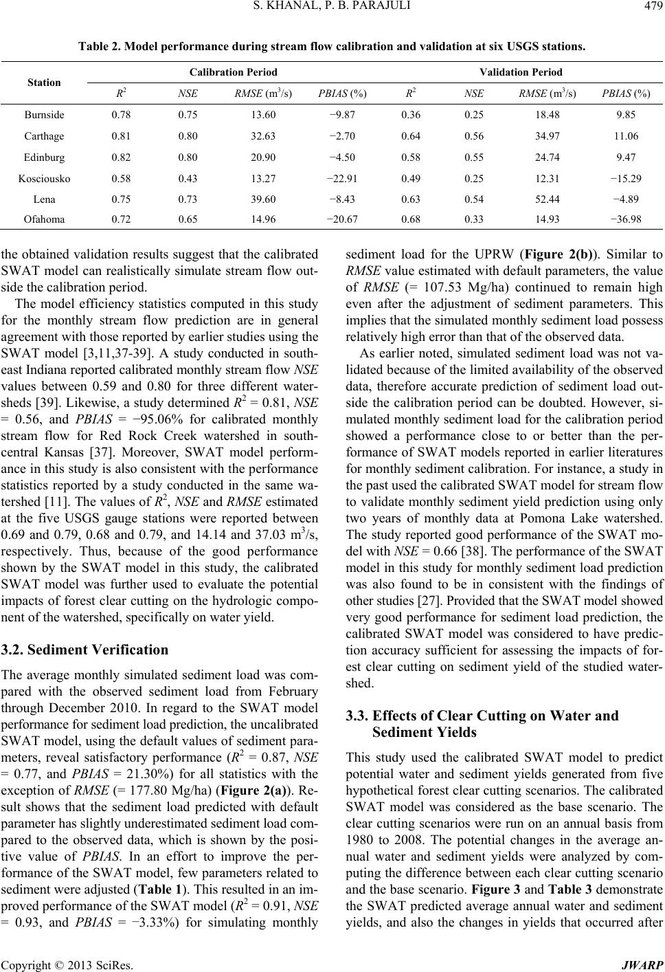 S. KHANAL, P. B. PARAJULI Copyright © 2013 SciRes. JWARP 479 Table 2. Model performance during stream flow calibration and validation at six USGS stations. Calibration Period Validation Period Station R2 NSE RMSE (m3/s) PBIAS (%) R2 NSE RMSE (m3/s) PBIAS (%) Burnside 0.78 0.75 13.60 −9.87 0.36 0.25 18.48 9.85 Carthage 0.81 0.80 32.63 −2.70 0.64 0.56 34.97 11.06 Edinburg 0.82 0.80 20.90 −4.50 0.58 0.55 24.74 9.47 Kosciousko 0.58 0.43 13.27 −22.91 0.49 0.25 12.31 −15.29 Lena 0.75 0.73 39.60 −8.43 0.63 0.54 52.44 −4.89 Ofahoma 0.72 0.65 14.96 −20.67 0.68 0.33 14.93 −36.98 the obtained validation results suggest that the calibrated SWAT model can realistically simulate stream flow out- side the calibration period. The model efficiency statistics computed in this study for the monthly stream flow prediction are in general agreement with those reported by earlier studies using the SWAT model [3,11,37-39]. A study conducted in south- east Indiana reported calibrated monthly stream flow NSE values between 0.59 and 0.80 for three different water- sheds [39]. Likewise, a study determined R2 = 0.81, NSE = 0.56, and PBIAS = −95.06% for calibrated monthly stream flow for Red Rock Creek watershed in south- central Kansas [37]. Moreover, SWAT model perform- ance in this study is also consistent with the performance statistics reported by a study conducted in the same wa- tershed [11]. The values of R2, NSE and RMSE estimated at the five USGS gauge stations were reported between 0.69 and 0.79, 0.68 and 0.79, and 14.14 and 37.03 m3/s, respectively. Thus, because of the good performance shown by the SWAT model in this study, the calibrated SWAT model was further used to evaluate the potential impacts of forest clear cutting on the hydrologic compo- nent of the watershed, specifically on water yield. 3.2. Sediment Verification The average monthly simulated sediment load was com- pared with the observed sediment load from February through December 2010. In regard to the SWAT model performance for sediment load prediction, the uncalibrated SWAT model, using the default values of sediment para- meters, reveal satisfactory performance (R2 = 0.87, NSE = 0.77, and PBIAS = 21.30%) for all statistics with the exception of RMSE (= 177.80 Mg/ha) (Figure 2(a)). Re- sult shows that the sediment load predicted with default parameter has slightly underestimated sediment load com- pared to the observed data, which is shown by the posi- tive value of PBIAS. In an effort to improve the per- formance of the SWAT model, few parameters related to sediment were adjusted (Table 1). This resulted in an im- proved performance of the SWAT model (R2 = 0.91, NSE = 0.93, and PBIAS = −3.33%) for simulating monthly sediment load for the UPRW (Figure 2(b)). Similar to RMSE value estimated with default parameters, the value of RMSE (= 107.53 Mg/ha) continued to remain high even after the adjustment of sediment parameters. This implies that the simulated monthly sediment load possess relatively high error than that of the observed data. As earlier noted, simulated sediment load was not va- lidated because of the limited availability of the observed data, therefore accurate prediction of sediment load out- side the calibration period can be doubted. However, si- mulated monthly sediment load for the calibration period showed a performance close to or better than the per- formance of SWAT models reported in earlier literatures for monthly sediment calibration. For instance, a study in the past used the calibrated SWAT model for stream flow to validate monthly sediment yield prediction using only two years of monthly data at Pomona Lake watershed. The study reported good performance of the SWAT mo- del with NSE = 0.66 [38]. The performance of the SWAT model in this study for monthly sediment load prediction was also found to be in consistent with the findings of other studies [27]. Provided that the SWAT model showed very good performance for sediment load prediction, the calibrated SWAT model was considered to have predic- tion accuracy sufficient for assessing the impacts of for- est clear cutting on sediment yield of the studied water- shed. 3.3. Effects of Clear Cutting on Water and Sediment Yields This study used the calibrated SWAT model to predict potential water and sediment yields generated from five hypothetical forest clear cutting scenarios. The calibrated SWAT model was considered as the base scenario. The clear cutting scenarios were run on an annual basis from 1980 to 2008. The potential changes in the average an- nual water and sediment yields were analyzed by com- puting the difference between each clear cutting scenario and the base scenario. Figure 3 and Table 3 demonstrate the SWAT predicted average annual water and sediment yields, and also the changes in yields that occurred after 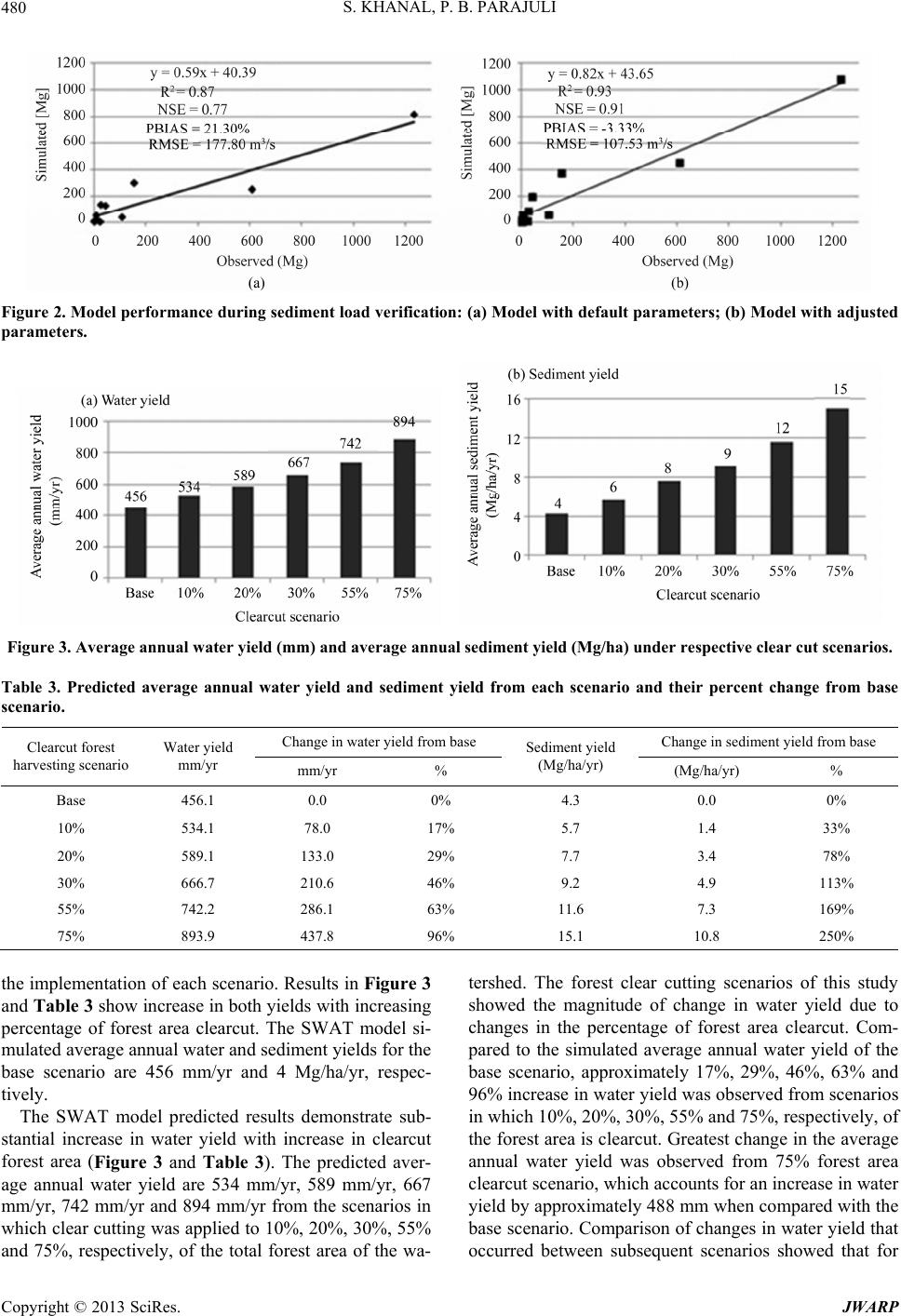 S. KHANAL, P. B. PARAJULI 480 Figure 2. Model performance during sediment load verification: (a) Model with default parameters; (b) Model with adjusted parameters. Figure 3. Average annual water yield (mm) and average annual sediment yield (Mg/ha) under respective clear cut scenarios. Table 3. Predicted average annual water yield and sediment yield from each scenario and their percent change from base scenario. Change in water yield from base Change in sediment yield from base Clearcut forest harvesting scenario Water yield mm/yr mm/yr % Sediment yield (Mg/ha/yr) (Mg/ha/yr) % Base 456.1 0.0 0% 4.3 0.0 0% 10% 534.1 78.0 17% 5.7 1.4 33% 20% 589.1 133.0 29% 7.7 3.4 78% 30% 666.7 210.6 46% 9.2 4.9 113% 55% 742.2 286.1 63% 11.6 7.3 169% 75% 893.9 437.8 96% 15.1 10.8 250% the implementation of each scenario. Results in Figure 3 and Ta ble 3 show increase in both yields with increasing percentage of forest area clearcut. The SWAT model si- mulated average annual water and sediment yields for the base scenario are 456 mm/yr and 4 Mg/ha/yr, respec- tively. The SWAT model predicted results demonstrate sub- stantial increase in water yield with increase in clearcut forest area (Figure 3 and Table 3). The predicted aver- age annual water yield are 534 mm/yr, 589 mm/yr, 667 mm/yr, 742 mm/yr and 894 mm/yr from the scenarios in which clear cutting was applied to 10%, 20%, 30%, 55% and 75%, respectively, of the total forest area of the wa- tershed. The forest clear cutting scenarios of this study showed the magnitude of change in water yield due to changes in the percentage of forest area clearcut. Com- pared to the simulated average annual water yield of the base scenario, approximately 17%, 29%, 46%, 63% and 96% increase in water yield was observed from scenarios in which 10%, 20%, 30%, 55% and 75%, respectively, of the forest area is clearcut. Greatest change in the average annual water yield was observed from 75% forest area clearcut scenario, which accounts for an increase in water yield by approximately 488 mm when compared with the base scenario. Comparison of changes in water yield that occurred between subsequent scenarios showed that for Copyright © 2013 SciRes. JWARP  S. KHANAL, P. B. PARAJULI 481 every 10% increase in the percentage of total forest area clearcut, the changes in water yield occurred between 55 mm to 78 mm. Similar change in model predicted aver- age annual water yield occurred, approximately by 76 mm, when the percentage of forest area clearcut was in- creased from 30% to 55%, which accounts for an in- crease of about 11% when compared with the 30% forest area clearcut scenario. A considerable change in average annual water yield of about 152 mm, an increase of ap- proximately 20%, was observed from 75% forest area clearcut scenario when compared with the 55% forest area clearcut scenario. Further, water yield generated from 75% forest area clearcut scenario is almost double the water yield from the base scenario. The SWAT model predicted sediment yield follows the similar pattern for the proposed clearcut scenarios (Figure 3 and Table 3). Percentage wise, increase in sediment yield from each scenario is much larger than the water yield, ranging between 33% and 250%. This suggests that the impact of clear cutting is greater on se- diment yield than that on water yield. In general, forest clear cutting increases the amount of water available for surface runoff due to increased water yield; therefore, increase in sediment yield after clear cutting can be attri- buted to an increase in water yield. The predicted sedi- ment yield ranged between 6 Mg/ha and 15 Mg/ha or 33% and 250%, respectively. Compared to the base value, 30% forest area clear cut scenario resulted in an increase of sediment yield by about 113% or 9 Mg/ha (Table 3). The predicted sediment yield generated from 55% forest clear cutting scenario is almost double the sediment yield generated from the base scenario. As expected, greatest increase in model predicted sediment yield was observed from 75% forest clear cutting scenarios, which resulted in an increase of about 250%, or 15 Mg/ha (Figure 3 and Table 3). Overall, this study supported the findings of earlier studies that have indicated that decrease in forest cover increases water and sediment yields [4,5,7]. If clear cut- ting is implemented in similar magnitude in the UPRW watershed, increase in average annual water and sedi- ment yields would occur by as much as 96% or 894 mm and 250% or 15 Mg/ha, respectively. However, due to unavailability of limited literatures from similar areas, cross validation of water and sediment yield generated from each scenario applied for the UPRW was not possi- ble. Further, it should be noted that the predicted yields from each scenario may be different than the actual yields in the watershed for similar magnitude of clear cutting. One possible explanation for the possible differ- ence in yields is the implementation of BMPs after clear cutting, which was beyond the scope of this study. An- other possible reason is the model uncertainty, which may exist due to different forest management activities at the local level, and also due to errors contained in the spatial data input. Thus, cautious interpretation of these results is suggested 4. Conclusions This study evaluated and compared the potential impacts of forest clear cutting on water and sediment yields of the UPRW located in east-central Mississippi. The SWAT model was used to simulate five hypothetical scenarios that represented clear cutting at 10%, 20%, 30%, 55% and 75% of the total forest area of the watershed. The SWAT model was first calibrated (1981-1995) and vali- dated (1996-2008) for monthly stream flow, and later verified (February 2010 to December 2010) for monthly sediment load. Results show that the SWAT model was able to simulate stream flow and sediment load satisfac- torily during the calibration/validation and verification period, respectively. This was shown by high R2 and NSE values (>0.6) at five of six stations during the calibration period. Small values of PBIAS (i.e. within the suggested limit of ±25% by earlier literatures) at all the six stations, and relatively small values of RMSE (13.27 - 39.60 m3/s) also reveal that the SWAT model was able to predict stream flow with minimum error and limited bias. Like- wise, R2 and NSE values greater than or equal to 0.77 for both default and adjusted sediment related parameters, PBIAS value within ±22% with default parameter and ±4% with adjusted parameter also illustrate that the SWAT model was able to predict sediment load reasona- bly well. The calibrated SWAT model was further used to simu- late the base scenario as well as the five clear cutting sce- narios. Potential changes in yields that may happen due to the implementation of clear cutting were computed by comparing yields from each scenario and a base scenario. As expected, increase in water and sediment yields was observed with increase in the percentage of forest area clear cut. This indicates that the SWAT model predicted results of this study have supported the findings of earlier studies that showed evidences supporting increase in wa- ter and sediment yields following forest clear cutting. Compared to the simulated average annual water yield of the base scenario, approximately 17%, 29%, 46%, 63% and 96% increase in water yield was observed from scenarios that represent clear cutting at 10%, 20%, 30%, 55% and 75%, respectively, of the total forest area of the watershed. These correspond to an average annual in- crease in water yield by approximately 78 mm, 133 mm, 210.6 mm, 286.1 mm and 437.8 mm from respective sce- narios. More seriously, an increase of about 33%, 78%, 113%, 169% and 250% was observed with increase in percentage of forest area clear cut. These represent an in- crease in average annual sediment yield by about 1.4 Mg/ha, 3.4 Mg/ha, 4.9 Mg/ha,, 7.3 Mg/ha, and 10.8 Copyright © 2013 SciRes. JWARP 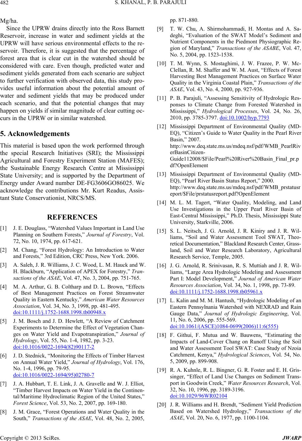 S. KHANAL, P. B. PARAJULI 482 Mg/ha. Since the UPRW drains directly into the Ross Barnett Reservoir, increase in water and sediment yields at the UPRW will have serious environmental effects to the re- servoir. Therefore, it is suggested that the percentage of forest area that is clear cut in the watershed should be considered with care. Even though, predicted water and sediment yields generated from each scenario are subject to further verification with observed data, this study pro- vides useful information about the potential amount of water and sediment yields that may be produced under each scenario, and that the potential changes that may happen on yields if similar magnitude of clear cutting oc- curs in the UPRW or in similar watershed. 5. Acknowledgements This material is based upon the work performed through the special Research Initiatives (SRI); the Mississippi Agricultural and Forestry Experiment Station (MAFES); the Sustainable Energy Research Centre at Mississippi State University; and is supported by the Department of Energy under Award number DE-FG3606GO86025. We acknowledge the contributions Mr. Kurt Readus, Assis- tant State Conservationist, NRCS/MS. REFERENCES [1] J. E. Douglass, “Watershed Values Important in Land Use Planning on Southern Forests,” Journal of Forestry, Vol. 72, No. 10, 1974, pp. 617-621. [2] M. Chang, “Forest Hydrology: An Introduction to Water and Forests,” 3rd Edition, CRC Press, New York. 2006. [3] A. Saleh, J. R. Williams, J. C. Wood, L. M. Hauck and W. H. Blackburn, “Application of APEX for Forestry,” Tran- sactions of the ASAE, Vol. 47, No. 3, 2004, pp. 751-765. [4] M. A. Arthur, G. B. Coltharp and D. L. Brown, “Effects of Best Management Practices on Forest Streamwater Quality in Eastern Kentucky,” American Water Resources Association, Vol. 34, No. 3, 1998, pp. 481-495. doi:10.1111/j.1752-1688.1998.tb00948.x [5] J. M. Bosch and J. D. Hewlett, “A Review of Catchment Experiments to Determine the Effect of Vegetation Chan- ges on Water Yield and Evapotranspiration,” Journal of Hydrology, Vol. 55, No. 1-4, 1982, pp. 3-23. doi:10.1016/0022-1694(82)90117-2 [6] J. D. Stednick, “Monitoring the Effects of Timber Harvest on Annual Water Yield,” Journal of Hydrology, Vol. 176, No. 1-4, 1996, pp. 79-95. doi:10.1016/0022-1694(95)02780-7 [7] J. A. Hubbart, T. E. Link, J. A. Gravelle and W. J. Elliot, “Timber Harvest Impacts on Water Yield in the Continen- tal/Maritime Hydroclimatic Region of the United States,” Forest Science, Vol. 53, No. 2, 2007, pp. 169-180. [8] J. M. Grace, “Forest Operations and Water Quality in the South,” Transactions of the ASAE, Vol. 48, No. 2, 2005, pp. 871-880. [9] T. W. Chu, A. Shirmohammadi, H. Montas and A. Sa- deghi, “Evaluation of the SWAT Model’s Sediment and Nutrient Components in the Piedmont Physiographic Re- gion of Maryland,” Transactions of the ASABE, Vol. 47, No. 5, 2004, pp. 1523-1538. [10] T. M. Wynn, S. Mostaghimi, J. W. Frazee, P. W. Mc- Clellan, R. M. Shaffer and W. M. Aust, “Effects of Forest Harvesting Best Management Practices on Surface Water Quality in the Virginia Coastal Plain,” Transactions of the ASAE, Vol. 43, No. 4, 2000, pp. 927-936. [11] P. B. Parajuli, “Assessing Sensitivity of Hydrologic Res- ponses to Climate Change from Forested Watershed in Mississippi,” Hydrological Processes, Vol. 24, No. 26, 2010, pp. 3785-3797. doi:10.1002/hyp.7793 [12] Mississippi Department of Environmental Quality (MD- EQ), “Citizen’s Guide to Water Quality in the Pearl River Basin,” 2007. http://www.deq.state.ms.us/mdeq.nsf/pdf/WMB_PearlRiv erBasinCitizen- Guide112008/$File/Pearl%20River%20Basin_Final_pr.p df?OpenElement [13] Mississippi Department of Environmental Quality (MD- EQ), “Pearl River Basin Status Report,” 2000. http://www.deq.state.ms.us/mdeq.nsf/pdf/WMB_prstatusr eport/$File/prstatusreport.pdf?OpenElement [14] M. L. M. Tagert, “Water Quality, Modeling, and Land Use Investigations in the Upper Pearl River Basin of East-Central Mississippi,” Ph.D. Thesis, Mississippi State University, Starkville, 2006. [15] S. L. Neitsch, J. G. Arnold, J. R. Kiniry and J. R. Wil- liams, “Soil and Water Assessment Tool SWAT, Theo- retical Documentation,” Blackland Research Center, Grass- land, Soil and Water Research Laboratory, Agricultural Research Service, Temple, 2005. [16] J. G. Arnold, R. Srinivasan, R. S. Muttiah and J. R. Wil- liams, “Large Area Hydrologic Modeling and Assessment Part I: Model Development,” Journal of American Water Resources Association, Vol. 34, No. 1, 1998, pp. 73-89. doi:10.1111/j.1752-1688.1998.tb05961.x [17] L. Kalin and M. M. Hantush, “Hydrologic Modeling of an Eastern Pennsylnania Watershed with NEXRAD and Rain Gauge Data,” Journal of Hydrologic Engineering, Vol. 11, No. 6, 2006, pp. 555-569. doi:10.1061/(ASCE)1084-0699(2006)11:6(555) [18] F. Githui, F. Mutua and W. Bauwens, “Estimating the Impacts of Land-Cover Chang on Runoff Using the Soil and Water Assessment Tool SWAT: Case Study of Nzoia Catchment, Kenya,” Hydrological Sciences, Vol. 54, No. 5, 2009, pp. 899-908. [19] R. A. Kuhnle, R. L. Bingner, G. R. Foster and E. H. Gris- singer, “Effect of Land Use Changes on Sediment Trans- port in Goodwin Creek,” Water Resources Research, Vol. 32, No. 10, 1996, pp. 3189-3196. doi:10.1029/96WR02104 [20] J. R. Williams and H. Brendt, “Sediment Yield Prediction Based on Watershed Hydrology,” Transactions of the ASAE, Vol. 20, No. 6, 1977, pp. 1100-1104. Copyright © 2013 SciRes. JWARP 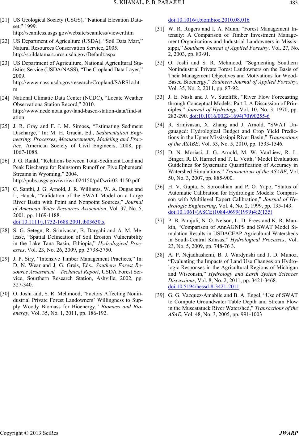 S. KHANAL, P. B. PARAJULI Copyright © 2013 SciRes. JWARP 483 [21] US Geological Society (USGS), “National Elevation Data- set,” 1999. http://seamless.usgs.gov/website/seamless/viewer.htm [22] US Department of Agriculture (USDA), “Soil Data Mart,” Natural Resources Conservation Service, 2005. http://soildatamart.nrcs.usda.gov/Default.aspx [23] US Department of Agriculture, National Agricultural Sta- tistics Service (USDA/NASS), “The Cropland Data Layer,” 2009. http://www.nass.usda.gov/research/Cropland/SARS1a.ht m [24] National Climatic Data Center (NCDC), “Locate Weather Observationa Station Record,” 2010. http://www.ncdc.noaa.gov/land-based-station-data/find-st ation [25] J. R. Gray and F. J. M. Simoes, “Estimating Sediment Discharge,” In: M. H. Gracia, Ed., Sedimentation Engi- neering: Processes, Meausurements, Modeling and Prac- tice, American Society of Civil Engineers, 2008, pp. 1067-1088. [26] J. G. Rankl, “Relations between Total-Sediment Load and Peak Discharge for Rainstorm Runoff on Five Ephemeral Streams in Wyoming,” 2004. http://pubs.usgs.gov/wri/wri024150/pdf/wrir02-4150.pdf [27] C. Santhi, J. G. Arnold, J. R. Williams, W. A. Dugas and L, Hauck, “Validation of the SWAT Model on a Large River Basin with Point and Nonpoint Sources,” Journal of American Water Resources Association, Vol. 37, No. 5, 2001, pp. 1169-1188. doi:10.1111/j.1752-1688.2001.tb03630.x [28] S. G. Setegn, R. Srinivasan, B. Dargahi and A. M. Me- lesse, “Spatial Delineation of Soil Erosion Vulnerability in the Lake Tana Basin, Ethiopia,” Hydrological Proc- esses, Vol. 23, No. 26, 2009, pp. 3738-3750. [29] J. P. Siry, “Intensive Timber Management Practices,” In: D. N. Wear and J. G. Greis, Eds., Southern Forest Re- source Assessment—Technical Report , USDA Forest Ser- vice, Sourthern Research Station, Ashville, 2002, pp. 327-340. [30] O. Joshi and, S. R. Mehmood, “Factors Affecting Nonin- dustrial Private Forest Landowners’ Willingness to Sup- ply Woody Biomass for Bioenergy,” Biomass and Bio- energy, Vol. 35, No. 1, 2011, pp. 186-192. doi:10.1016/j.biombioe.2010.08.016 [31] W. R. Rogers and I. A. Munn, “Forest Management In- tensity: A Comparison of Timber Investment Manage- ment Organizations and Industrial Landowners in Missis- sippi,” Southern Journal of Applied Forestry, Vol. 27, No. 2, 2003, pp. 83-91. [32] O. Joshi and S. R. Mehmood, “Segmenting Southern Nonindustrial Private Forest Landowners on the Basis of Their Management Objectives and Motivations for Wood- Based Bioenergy,” Southern Journal of Applied Forestry, Vol. 35, No. 2, 2011, pp. 87-92. [33] J. E. Nash and J. V. Sutcliffe, “River Flow Forecasting through Conceptual Models: Part I. A Discussion of Prin- ciples,” Journal of Hydrology, Vol. 10, No. 3, 1970, pp. 282-290. doi:10.1016/0022-1694(70)90255-6 [34] R. Srinivasan, X. Zhang and J. Arnold, “SWAT Un- gauaged: Hydrological Budget and Crop Yield Predic- tions in the Upper Mississippi River Basin,” Transactions of the ASABE, Vol. 53, No. 5, 2010, pp. 1533-1546. [35] D. N. Moriasi, J. G. Arnold, M. W. VanLiew, R. L. Binger, R. D. Harmel and T. L. Veith, “Model Evaluation Guidelines for Systematic Quantification of Accuracy in Watershed Simulations,” Transactions of the ASABE, Vol. 50, No. 3, 2007, pp. 885-900. [36] H. V. Gupta, S. Sorooshian and P. O. Yapo, “Status of Automatic Calibration for Hydrologic Models: Compari- son with Multilevel Expert Calibration,” Journal of Hy- drologic Engineering, Vol. 4, No. 2, 1999, pp. 135-143. doi:10.1061/(ASCE)1084-0699(1999)4:2(135) [37] P. B. Parajuli, N. O. Nelson, L. D. Frees and K. R. Man- kin, “Comparison of AnnAGNPS and SWAT Model Si- mulation Results in USDACEAP Agricultural Watersheds in South-Central Kansas,” Hydrological Processes, Vol. 23, No. 5, 2009, pp. 748-76 3. [38] A. P. Nejadhashemi, B. J. Wardynski and J. D. Munoz, “Evaluating the Impacts of Land Use Changes on Hydro- logic Responses in the Agricultural Regions of Michigan and Wisconsin,” Hydrology and Earth System Sciences Discussions, Vol. 8, No. 2, 2011, pp. 3421-3468. doi:10.5194/hessd-8-3421-2011 [39] G. G. Vazquez-Amabile and B. A. Engel, “Use of SWAT to Compute Groundwater Table Depth and Stream Flow in the Muscatatuck River Watershed,” Transactions of the ASAE, Vol. 48, No. 3, 2005, pp. 991-1003
|