Journal of Electromagnetic Analysis and Applications
Vol.6 No.1(2014), Article ID:42208,10 pages DOI:10.4236/jemaa.2014.61003
Numerical Modeling of Electromagnetic Scattering from Sea Surface Covered by Oil
Lab-STICC UMR CNRS 6285, ENSTA Bretagne, 2, Rue François Verny, 29806, Brest Cedex 09, France.
Email: Helmi.Ghanmi@ensta-bretagne.fr, Ali.Khenchaf@ensta-bretagne.fr, Fabrice.Comblet@ensta-bretagne.fr
Received November 1st, 2013; revised December 2nd, 2013; accepted December 29th, 2013
ABSTRACT
The aim of this work is to study the impacts of the oil spills on the electromagnetic scattering of the ocean surfaces in bistatic and monostatic configurations. Therefore, in this paper, we will study the influence of the pollutants (oil spills) on the physical and geometrical properties of sea surface. In recent literature, the study of the electromagnetic scattering from contaminated sea surface (sea surface covered by oil spill) was limited in monostatic case. In this paper, we will study this effect in bistatic configuration, which is interested in presence of pollution in sea surface. Indeed, we will start the numerical analysis of the bistatic scattering coefficients of a clean sea surface. Then, we will study the electromagnetic signature from sea surface covered by oil spills in bistatic case using the numerical Forward-Backward Method (FBM). The obtained numerical simulation of bistatic scattering coefficients of clean and contaminated sea surface is studied as a function of various parameters (frequency, incident angle, sea state, type of pollutant…). And the obtained results are also compared with those published in the literature, including those using asymptotic methods.
Keywords:Sea Surface; Oil Spills; Forward-Backward Method; Asymptotic Methods; Electromagnetic Scattering Coefficients; Bistatic Configuration
1. Introduction
In the maritime environment, the presence of objects, ship wake and pollutants changes the physical and geometrical properties of sea surface. In this paper, a spatial focus is given to analyze the electromagnetic signature of pollutants such as organic films, petrol and oil slicks. To date, many systems have been developed such as SAR (Synthetic Aperture Radar) to detect the presence of the oil spill on the sea surface (Figure 1). To improve the performance of existing systems, it becomes very important to analyze in greater detail the information contained in the electromagnetic field scattered by the sea surface [1-3]. In this context, modeling the interaction of electromagnetic waves with polluted seas or not takes all its importance. In particular, the estimation of the electromagnetic scattering based on geometric (roughness) and physical (dielectric properties of sea water with or without pollutant) properties of the ocean surface is an essential tool in the design of detection systems, in particular for pollutant [4].
In recent years, many research works have focused on modelling the electromagnetic scattering from ocean surface. Indeed, on one hand, different models based on the geometric description of the sea surface (Elfouhaily spectrum and Pierson-Moskowitz spectrum) [5,6] and on the other hand, different electromagnetic models have been developed for studying the electromagnetic scattering from sea surface. The existing electromagnetic models are classified into: approximate methods like the Kirchhoff Approximation (KA), Small Perturbation Method (SPM), Two Scale Model (TSM), Small Slope Approximation (SSA) [7-9] and exact methods such as the finite difference time domain (FDTD) [10], Finite Element Method (FEM) [11], Method of Moment (MoM) [12], Forward-Backward Method (FBM), Forward-
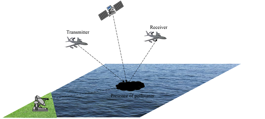
Figure 1. Electromagnetic detection of oil spills on sea surfaces.
Backward Method with Spectral Accelerate Algorithm (FBM/SAA) [13-17].
In our study, the numerical FBM method is used to calculate the bistatic scattering coefficients from a clean and a polluted sea surface. Recently in [4], the study of the electromagnetic scattering from ocean surface covered by oil spills was performed in monostatic case by using the numerical method of moment and Monte-Carlo simulation. The contribution of this paper is the study of this effect in bistatic case (Forward propagation configuration), which is interested in presence of pollution in sea surface. We will start the numerical simulation of the oil spills effect on the sea surface. Then, we represent our numerical results of the bistatic scattering coefficients from a clean and polluted sea surface by using the numerical Forward-Backward method.
This paper is organized as follows: in the first part, we present the impact of the oil spills on the surface height spectrum of a rough sea surface. To characterize the clean sea surface, the model of Elfouhaily et al. [6] is used, and for the contaminated sea surface we use the Lombardini et al. model [18]. In the second part, we discuss the calculation method of electromagnetic scattering coefficients (FBM). In the last part, by using the FBM method, we present the numerical results of electromagnetic scattering coefficients obtained for non-polluted and polluted sea surface.
2. Formulations
2.1. Sea Surface Description
In our simulation, we use the Elfouhaily model for sea roughness spectrum [6]. This sea spectrum formulation is given in the form:
 (1)
(1)
 represents the isotropic part of the Elfouhaily spectrum modulated by the angular function
 .
.  is the sea wave number and
 ![]() is the wind direction. Figure 2 illustrates the omnidirectional spectrum and the angular function for different values of the wind speed.
is the wind direction. Figure 2 illustrates the omnidirectional spectrum and the angular function for different values of the wind speed.
In this section, we study the effect of the oil spills on the geometrical properties of the sea surface (ocean spectrum). We will focus on the oil from a layer up the sea surface (contaminated sea surface). Then we present its influence on the ocean spectrum using a damping model [18], and we compared the obtained results with the representation of clean sea surface spectrum.
According to Lombardini et al., the influence of the pollution is introduced in the form of an attenuation coefficient applied to the clean sea spectrum:
 (2)
(2)
This damping effect is expressed by the attenuation coefficient explicitly given by the following equation:
 (3)
(3)
where
 (4)
(4)
A dimensional quantities and
 (5)
(5)
The dispersion law, ![]() denotes the clean sea spectrum,
denotes the clean sea spectrum, ![]() the polluted sea spectrum,
the polluted sea spectrum,  the sea water density,
 ![]() the kinematic viscosity,
the kinematic viscosity, ![]() the surface tension,
the surface tension, ![]() acceleration of gravity,
acceleration of gravity,  the wave number,
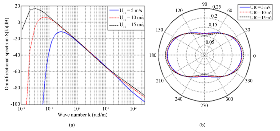
Figure 2. Elfouhaily spectrum with different values of the wind speed: (a) Omnidirectional spectrum (b) Angular function.
 the elasticity modulus and
  is a characteristic pulsation which for soluble film depends upon the diffusional relaxation and for insoluble films, depends upon structural relaxation between intermolecular forces. In Equation (3) a plus sign indicate soluble films, while a minus sign refers to insoluble films. In this paper we will focus a 1- D rough sea surface contaminated by insoluble films.
In general the damping ratio should not be directly interpreted as corresponding to Equation (3). It would be noted so if the film was uniformly dispersed by wind and waves, so that the surface investigated results only partially covered by the film. In this case we shall introduce a fractional filling factor, F i.e., the ratio for the surface covered by film with respect to the total area considered, and write for the damping ratio (2) the expression:
 (6)
(6)
Figure 3 presents the damping ratio variation with frequency for different fractional filling factors.
In this paper we will focus on one-dimensional rough sea surface covered by of insoluble films (fully covered sea, F = 1). Figure 4 shows the comparison between the height spectrum of clean sea surface and the polluted sea surface. The normalized height spectrum of contaminated sea surface (sea surface covered by oil film) is plotted for different parameters of oil film [18]. It was observed that the attenuation due to pollutant film is essentially located at the high frequencies, which corresponds to the capillary waves.
In the next section we will present the numerical FBM method used to calculate the electromagnetic scattering coefficients of clean and polluted ocean surface.
2.2. Numerical Forward-Backward Method
Many approaches were developed to estimate the electromagnetic scattering from sea surface (The asymptotic models and the numerical exact methods). Each of asymptotic methods is an approximation and is based on particular conditions (SPM covers the small-scale roughness; KA is valid for a surface with wide-scale roughness). However, the numerical exact methods are valid for all scale of roughness and give more precise results. Among the exact methods, in our study the numerical FBM method is used to calculate the bistatic scattering coefficients from a clean and a polluted sea surface. It should be noted that the chosen method (FBM) in this paper has already been applied, in particular to calculate the electromagnetic signature of a breaking wave, and the results obtained in this context were compared with measurements made in the anechoic chamber with profiles of breaking waves in aluminum [19,20].
In this work, the presented simulations of electromagnetic scattering coefficients of clean and contaminated sea surface are mainly based on a Forward-Backward Method. The FBM method split the surface current into contributions; one is the forward component (the courant contribution due to the waves propagating forwards) and another is the backward component (The current contribution due to the waves propagating backwards). This method has been developed to calculate the scattering coefficients from dielectric rough surface [16]. Furthermore, to accelerate this method and to treat a large problem, the FBM method was combined with Spectral Accelerate Algorithm (FBM/SAA) [15,17].
The FBM method has been well-discussed in [13-17]. The surface electric and magnetic fields can be evaluated by solving the following pair of integral equations:
 (7)
(7)
where ![]() is the incident wave,
is the incident wave,  is the induced current in the surface, the fields
  in the upper medium (free space) and
  in the lower medium,
  and
and  are respectively the permeability of the free space and the lower medium,
 ![]() is the radian frequency,
is the radian frequency,  and
and  are the source and observation points respectively,
  the outgoing normal to the surface
  and
and  are respectively, the two dimensional Green function in the free space and in the lower medium.
The integral Equation (7) are discrete under a matrix
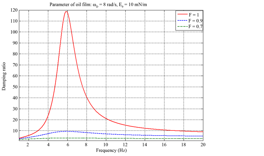
Figure 3. Damping ratio for different fractional filling factors.
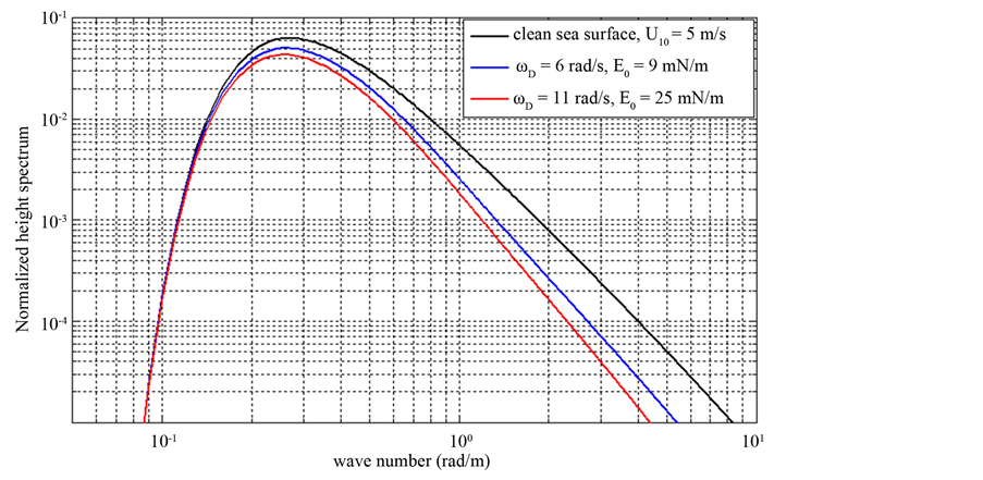
Figure 4. Comparaison between a clean and oil spilled sea surface.
form (8) by using rectangular pulse basis functions and the point matching technique:
 (8)
(8)
where  is the impedance matrix,
  is the wave incidence and
  is the induced current along the rough surface. In the FBM approach, the matrix of Equation (8) is decomposed as:
![]() (9)
(9)
![]() (10)
(10)
Equation (8) can be now decomposed into forward propagation and backward propagation of matrix equations, respectively as follows:
 (11)
(11)
This system of equation can be solved iteratively; indeed the currents ,
,  at the i-th iteration can be obtained as
 (12)
(12)
The algorithm begins with .
.
After competition of the surface current, so that we can calculate the scattered field from the non-polluted and polluted sea surface. Using the Monte Carlo technique, we calculate the overage of the bistatic scattering coefficients.
Finally, the algorithm of FBM method used in this paper is adapted to estimate the electromagnetic scattering coefficients from clean or polluted rough sea surface.
In the next part, first we study the electromagnetic scattering from non-polluted sea surface and we will present the outcomes of the pollutant film on the electromagnetic sea surface scattering.
3. Numerical Analysis of Bistatic Scattering Of Contaminated Rough Sea Surface by Using The Forward-Backward Method
Many works [21-]">23] show that the FBM method and the accelerated version FBM-SAA is interesting for maritime applications (ship target, electromagnetic scattering from braking wave). However, there are not research works, which analyze the oil spills effect on the electromagnetic signature of sea surface observed in bistatic configuration and by using the numerical FBM method. This is the object of this section.
In this section, we will focus on electromagnetic scattering coefficients of ocean surface covered by oil spills. First, we study the case of one-dimensional rough sea surface (clean sea surface without pollutants). By using the numerical FBM method, we realize the numerical simulation of the bistatic scattering coefficients (in forward propagation configuration) of clean rough sea surface, and we compare the numerical results with those obtained by using the asymptotic models such as small perturbation method (SPM) [7,]">24]. This step will allow to validate the results obtained by the developed model, and to have a reference on an ocean surface without oil spills.
3.1. Comparison with Asymptotic Methods
In this part, by using the FBM method, we present numerical simulations of bistatic scattering coefficients (in forward propagation configuration) of clean rough sea surface, and we compare the numerical results with those obtained by using the asymptotic methods, especially with those given by the small perturbation method (SPM). In this simulation the sea surface is assumed to be dielectric rough surface. Figure 5 compares the results obtained using the numerical FBM method with those given by using SPM model in the forward propagation configuration. The parameters are fixed as follows: The electromagnetic wave frequency is 10 GHz (X band), the relative dielectric constant of sea is (55.5 + i38), the incident angle is fixed to θi = 60˚, and the wind speed U10 = 5 m/s.
Using the Monte-Carlo technique, we calculate the average of the bistatic scattering coefficients (60 realizations).
We compared the results obtained by FBM with those given by SPM method; we can notice that the results obtained by using the numerical FBM method are in good agreements with those given by the asymptotic approach SPM. It should be noted that the SPM method is accurate for the rough sea surfaces with the small roughness conditions (valid for a slightly rough sea surface). In our future works we will compared the numerical FBM method with other asymptotic models such as (TSM, SSA, WCA…) which have a wider application domain than the SPM method.
3.2. Bistatic Scattering Coefficients of Sea Surface Contaminated by Oil
To analyze the influence of the oil pollutants on the electromagnetic signature from sea surface, we represented the variation of the bistatic scattering coefficients (in forward propagation configuration) under different conditions of sea state, frequencies, type of pollutant, and incidence angles. Figure 6 gives the bistatic scattering coefficients for both clean and polluted surface by using the FBM method. The sea surface is described by using the Elfouhaily spectrum, the wind speed U10 = 5 m/s, the
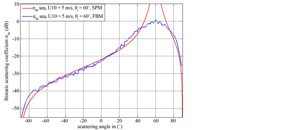
Figure 5. Bistatic scattering comparison of numerical method (FBM) and (SPM): frequency (10 GHz) and incidence angle (60˚).
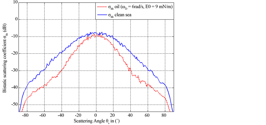
Figure 6. Bistatic scattering coefficients of clean and contaminated sea surface: frequency (3 GHz) and incidence angle (0˚).
sea temperature and salinity are respectively T = 20˚C and S = 35 ppt the frequency is 3 GHz (S band), the incident angle is fixed to θi = 0˚, HH polarizations, and the scattering angle in vary from −90˚ to 90˚. The pollutant is considered insoluble film and its relative dielectric constant is (2.25 + i0.01) [22], and the relative dielectric constant of the sea water is equal to (70.5 + i40) [21].
Figures 7-9 show the bistatic scattering coefficients of the clean and the contaminated rough sea surface obtained for incidence angle equal to 40˚, 70˚ and 80˚ respectively. The other parameters are the same as those given in Figure 6.
From Figures 6-9 it may be noted the differences between the scattering coefficients of the clean and the polluted sea surface. Indeed, for the incidence angle equal to 0˚ (Figure 6) the differences exist for both negative and positive scatterings angles, whereas for the incidence angles 40˚, 70˚ and 80˚ (Figures 7-9) the differences appear at negative scattering angles, more precisely in the range [−90˚, θi = θs]. The deviation between the scattering coefficients is essentially due to both the influence of pollutant in surface height spectrum and relative dielectric constant of the pollutant.
In order to obtain more information about the deviation between the scattering coefficients of oil spilled sea surface and the non polluted surface, we present in Figures 10 and 11 another comparison at Ku band (frequency is 14 GHz).
In Figures 10 and 11 the electromagnetic wave frequency is 14 GHz (Ku band), the dielectric constant of
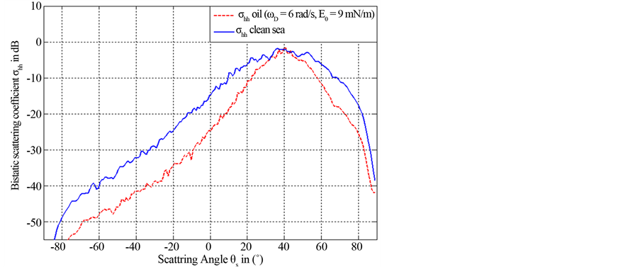
Figure 7. Bistatic scattering coefficients of clean and contaminated sea surface: frequency (3 GHz) and incidence angle (40˚).
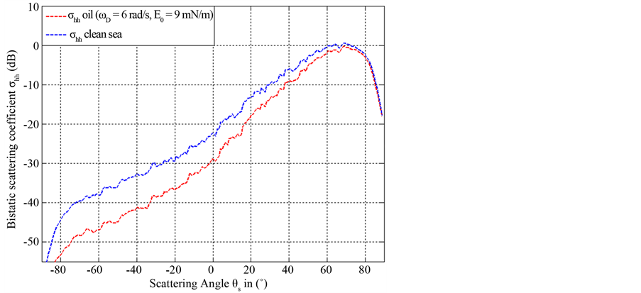
Figure 8. Bistatic scattering coefficients of clean and contaminated sea surface: frequency (3 GHz) and incidence angle (70˚).

Figure 9. Bistatic scattering coefficients of clean and contaminated sea surface: frequency (3 GHz) and incidence angle (80˚).
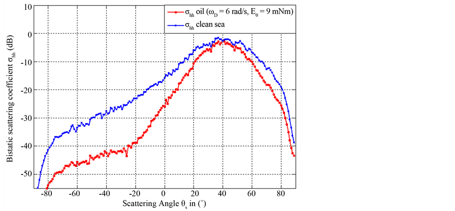
Figure 10. Bistatic scattering coefficients from clean and contaminated sea surface: frequency (14 GHz) and incidence angle (40˚).
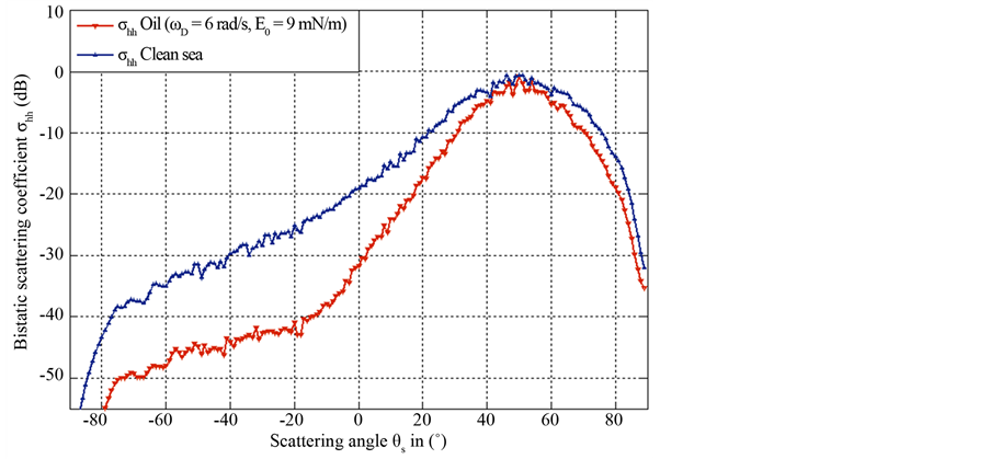
Figure 11. Bistatic scattering coefficients from clean and contaminated sea surface: frequency (14 GHz) and incidence angle (50˚).
sea surface is (45.75 + i39) , the incident angle is equal to 40˚ in Figure 10 and to 50˚ in Figure 11 and the other parameter are the same as in Figure 6.
By comparing Figures 7 and 10, we notice that for Ku band (frequency is fixed to 14 GHz) the difference between the electromagnetic scattering coefficients of the clean and polluted sea surface is greater than S band (frequency 3 GHz). From these analyses, we can conclude the influence of the oil spills on the electromagnetic signature of ocean surface is more important at a higher frequency.
In our study, the numerical simulations of electromagnetic scattering coefficients from both clean and polluted sea surface are limited to the problem of one dimensional surface (1D) and only the cross-polarization scattering coefficients can be evaluated by using the numerical FBM method. The main purpose of our future works is to evaluate the co-polarization and cross-polarization scattering by tow-dimensional rough sea surface (clean and oil-spilled sea surface) in bistatic configuration.
4. Conclusions
In this paper, by using the numerical FBM method, the EM scattering by clean and polluted rough sea surface observed in bistatic case (forward propagation configuration) is investigated. For clean rough sea surface, the numerical results obtained by using FBM were compared with those given by using the asymptotic methods (small perturbation method-SPM). The pollutant effect on sea surface spectrum and in the electromagnetic scattering coefficients was described and modeled for various conditions of sea surface, frequencies and incidence angles.
Comparing the scattering coefficients of the clean sea surface with those of polluted sea surface, it may be noted the differences between the scattering coefficients. These results demonstrate the influence of the pollution on the electromagnetic signature of the sea surface.
The objective of future work is to compare the performance of the FBM method with other asymptotic models such as (TSM, SSA, WCA…) which have a large validity domain than the small perturbation method (SPM). And we will study the electromagnetic scattering from other geometric configurations of observation and other types of surface (including 2D dielectric rough sea surface).
Acknowledgments
The authors wish to thank the EU for its support to NETMAR project where this work is in progress and they also would like to thank the other partners of NETMAR project, and also the “Région Bretagne” for its support.
REFERENCES
- G. Franceschetti, A. Iodice, D. Riccio, G. Ruello and R. Siviero, “SAR Raw Signal Simulation of Oil Slicks in Ocean Environments,” Transactions on Geoscience Remote Sensing, Vol. 40, No. 9, 2002, pp. 1935-1949. http://dx.doi.org/10.1109/TGRS.2002.803798
- C. Brekke and A. H. S. Solberg, “Oil Spill Detection by Satellite Remote Sensing,” Remote Sensing of Environment, Vol. 95, No. 1, 2005, pp. 1-13. http://dx.doi.org/10.1016/j.rse.2004.11.015
- A. H. S.Solberg, “Remote Sensing of Ocean Oil-Spill Pollution,” Proceeding of the IEEE, Vol. 100, No. 10, 2012, pp. 2931-2945. http://dx.doi.org/10.1109/JPROC.2012.2196250
- C.-S. Yang, P. Seong-Min, O. H. Yisok and O. Kazu, “An Analysis of the Radar Backscatter from Oil-Covered Sea Surfaces Using Moment Method and Monte-Carlo Simulation: Preliminary Results,” Acta Oceanologica Sinica, Vol. 32, No. 1, 2013, pp. 59-67. http://dx.doi.org/10.1007/s13131-013-0267-7
- E. I. Thorsos, “Acoustic Scattering from a ‘PiersonMoskowitz’ Sea Surface,” Journal of the Acoustical Society of America, Vol. 88, No. 1, 1990, pp. 335-349. http://dx.doi.org/10.1121/1.399909
- T. Elfouhaily, B. Chapron and K. Katsaros, “A Unified Directional Spectrum for Long and Short Wind-Driven Waves,” Journal of Geophysical research, Vol. 102, No. C7, 1997, pp. 15781-15796. http://dx.doi.org/10.1029/97JC00467
- A. Khenchaf, “Bistatic Scattering and Depolarization by Randomly Rough Surface: Application to Natural Rough Surface in X-Band,” Wave in Random and Complex Media, Vol. 11, No. 2, 2000, pp. 61-87. http://dx.doi.org/10.1088/0959-7174/11/2/301
- A. Awada, Y. Ayari, A. Khenchaf and A. Coantanhay, “Bistatic Scattering from an Anisotropic Sea Surface: Numerical Comparison between the First-Order SSA and the TSM models,” Wave in Random and Complex Media, Vol. 16, No. 3, 2006, pp. 383-394. http://dx.doi.org/10.1080/17455030600844089
- A. G. Voronovich, “Small Slope Approximation in Wave Scattering from Rough Surfaces,” Soviet Physics-JETP, Vol. 62, 1985, pp. 65-70.
- A. Taflove and M. Brodwin, “Numerical Solution of Steady-State Electromagnetic Scattering Problems Using the Time-Dependant Maxwell’s Equations,” IEEE Transactions on the Microwave Theory and Techniques, Vol. 23, No. 8, 1975, pp. 623-630. http://dx.doi.org/10.1109/TMTT.1975.1128640
- Y. Q. Jin, and G. Li, “Detection of a Scatter Traject over Randomly Rough Surface by Using Angular Correlation Function in Finite Element Approach,” Wave in Random Media, Vol. 10, No. 2, 2000, pp. 273-280. http://dx.doi.org/10.1080/13616670009409774
- R. F. Harrington, “Field Computation by Moment Method,” IEEE Press, New York, 1993. http://dx.doi.org/10.1109/9780470544631
- D. Holliday, L. L. DeRaad Jr. and G. J. St-Cyr, “ForwardBackward: A New Method for Computing Low-Grazing Angle Scattering,” IEEE Transactions on Antennas and Propagation, Vol. 44, No. 5, 1996, pp. 722-729. http://dx.doi.org/10.1109/8.496263
- D. Holliday, L. L. DeRaad Jr. and G. J. St-Cyr, “ForwardBackward for Scattering from Imperfect Conductor,” IEEE Transactions on Antennas and Propagation, Vol. 46, No. 1, 1998, pp. 101-107. http://dx.doi.org/10.1109/8.655456
- H. T. Chou and J. T. Jhonson, “Formulation of ForwardBackward Method Using Novel Spectral Acceleration for the Modeling of Scattering from Impedance Rough Surfaces,” IEEE Transactions on Geoscience and Remote Sensing, Vol. 38, No. 1, 2000, pp. 605-607. http://dx.doi.org/10.1109/36.823954
- A. Iodice, “Forward-Backward Method for Scattering from Dielectric Rough Surfaces,” IEEE Transactions on Antennas and Propagation, Vol. 50, No. 7, 2002, pp. 901-911. http://dx.doi.org/10.1109/TAP.2002.800700
- Z.-X. Li, “Bistatic Scattering from Rough Dielectric Soil Surface with a Conducting Object Partially Buried by Using the GFBM/SAA Method,” IEEE Transactions on Antennas and Propagation, Vol. 54, No. 7, 2006, pp. 2072-2080. http://dx.doi.org/10.1109/TAP.2006.877187
- P. P. Lombardini, B. Fiscella, P. Trivero, C. Cappa and W. D. Garrett, “Modulation of the Spectra of Short Gravity Waves by Sea Surface Films: Slick Detection and Characterization with a Microwave Probe,” Journal of Atmospheric and Oceanic Technology, Vol. 6, No. 6, 1989, pp. 882-890. http://dx.doi.org/10.1175/1520-0426(1989)006<0882:MOTSOS>2.0.CO;2
- S. E. Ben Khadra and A. Khenchaf, “The Bistatic Electromagnetic Signature of Heterogeneous Sea Surface: Study of the Hydrodynamic Phenomena,” Proceedings of International Conference of the IEEE Goescience RemoteSensing, Honolulu, 25-30 July 2010, pp. 3549-3552. http://dx.doi.org/10.1109/IGARSS.2010.5652177
- S. B. Khadra, A. Khenchaf and K. B. Khadhra, “Numerical and Experimental Study of the Hydrodynamic Phenomena in Heterogeneous Sea Surface, EM Bistatic Scattering,” Progress in Electromagnetics Research B, Vol. 35, 2011, pp. 151-166. http://dx.doi.org/10.2528/PIERB11092003
- T. Meissner and F. J. Wentz, “The Complex Dielectric Constant of Pure and Sea Water from Microwave Satellite Observations,” IEEE Transactions on Geoscience and Remote Sensing, Vol. 42, No. 9, 2004, pp. 1836-1849. http://dx.doi.org/10.1109/TGRS.2004.831888
- T. Friizo, Y. Schildberg, O. Rambeau, T. Tjomsland, H. Fordedal and J. Sjoblom, “Complex Permittivity of Crude Oils and Solutions of Heavycrude Oils Fractions,” Journal of Dispersion Science and Technology, Vol. 19, No. 1, 1998, pp. 93-126. http://dx.doi.org/10.1080/01932699808913163
- Y. Q. Jin and Z. X. Li, “Numerical Simulation of Radar Surveillance for the Ship Target and Oceanic Clutters in Two-Dimensional Model,” Radio Science, Vol. 38, No. 3, 2003, pp. 1045-1050. http://dx.doi.org/10.1029/2002RS002692
- M. Y. Ayari, A. Coatanhay and A. Khenchaf, “The Influence of Ripple Damping on Electromagnetic Bistatic Scattering by Sea Surface,” Proceedings of International Conference of the IEEE IGARSS’05, Seoul, 25-29 July 2005, pp. 1345-1348. http://dx.doi.org/10.1109/IGARSS.2005.1525370