Journal of Electromagnetic Analysis and Applications
Vol. 3 No. 9 (2011) , Article ID: 7456 , 9 pages DOI:10.4236/jemaa.2011.39057
Time Domain Modeling of Powerline Impulsive Noise at Its Source
![]()
1Orange Labs, Lannion, France; 2Innovas, Lannion, France; 3University of Nantes, Saint Nazaire, France.
Email: hassina.chaouche@gmail.com
Received July 14th, 2011; revised August 12th, 2011; accepted August 21st, 2011.
Keywords: Powerline Communication, Impulsive Noise Modeling, Electrical Appliances
ABSTRACT
Noise characteristics of an indoor power line network strongly influence the link capability to achieve high data rates. The appliances shared with PLC modems in the same powerline network generate different types of noises, among them the impulsive noises are the main source of interference resulting in signal distortions and bit errors during data transmission. With regard to impulsive noise many models were proposed in the literature and shared the same impulsive noise definition: “unpredictable noises measured in the receiver side”. Authors are, consequently, confronted to model thousands of impulsive noises whose plurality would very likely come from the diversity of paths that the original impulsive noise took. In this paper, an innovative modelling approach is applied to impulsive noises which are studied here directly at their sources. Noise at receiver would be simply the noise model at source convolved by powerline channel block. In the new analytical model, the impulsive noise at source is described by a succession of short pulses, each modeled by a phase-shifted Gaussian. Noises at source are classified into 6 different classes [1], and a noise generator is established for each class.
1. Introduction
PLC channel is characterized by its several differences from other wired media, as its interference and noise levels are much larger. Understanding of complete characteristics of broadband PLC channel is important when developing PLC transmission chains [2,3] and simulating the performance of advanced communication technologies [4,5].
Due to the multiple appliances connected to the network, the transfer function between a transmitter and a receiver is strongly affected by multi path [6,7] and thus is frequency dependant. Based either on measurements or on the network topology, many channel models have been proposed [6-14].
The appliances shared with PLC modems in the same powerline network generate noises which are stationary, cyclo-stationary or impulsive [15].
Impulsive noise is the main source of interference which causes signal distortions leading to bit errors while data transmission. Origins of impulsive noises are multiple: power switches, power supplies, and generally speaking domestic appliances.
Several approaches have been followed for characterizing the PLC impulsive noise in the time domain. In [16,17] and [18] the proposed models are based on noise classification according to duration, bandwidth and of inter-arrival intervals between impulses. Based on Middleton and Markov modeling of the impulsive noise, examples of the relationships between time and frequency domains are shown in [19].
The proposed models share the same impulsive noise definition: “unpredictable noises measured in the receiver side”. Authors are, consequently, confronted to model thousands of impulsive noises whose plurality would very likely come from the diversity of paths that the original impulsive noise took.
In this paper, an innovative modeling approach is applied to impulsive noises which are henceforth studied directly at their sources outputs. Noise at receiver would be simply the noise model at source convolved by powerline Channel Transfer Function (CTF). CTF model examples can be found in [11] and [14].
Measuring impulsive noises at source has many advantages:
-Much less noises to model.
-Ability to correlate with noise generators.
-Much easily classifiable.
This paper is organized as follows: Section 2 presents the analytical model and a time domain noise generator is detailed. Then the proposed model is validated by comparison to measured noises. Finally, a modelling of inter-arrivals between noise events is proposed in Section 3, which could be useful if a model of impulsive noise at source over a large time scale is needed. A conclusion closes the paper in the last section.
2. Modelling of Impulsive Noise at Its Source
In previous paper [1], a characterization of impulse noise at source has been achieved. Measurements are carried out in the time domain, by means of a digital oscilloscope, as shown in the block diagram of Figure 1.
The device under test is isolated from the remaining electrical network by means of a Line Impedance Stabilization Network (LISN). The experiment is conducted in a semi anechoic room in order to avoid external radio coupling.
For each device, impulsive noise is recorded for 50ms when its amplitude exceeds a pre-defined threshold that depends on the stationary noise amplitude.
The noise is recorded simultaneously on two scope channels with different sensitivities. This makes it possible to reach a good sensitivity for the weak noise samples and not to clip the strong amplitude samples of the noise. The sampling rate is fixed to 250 Mega Samples per second.
The PLC impulsive noise is generated by 23 different domestic appliances Six classes of noises have also been distinguished:
- Class 1: Electrical switch and thermostat ON event.
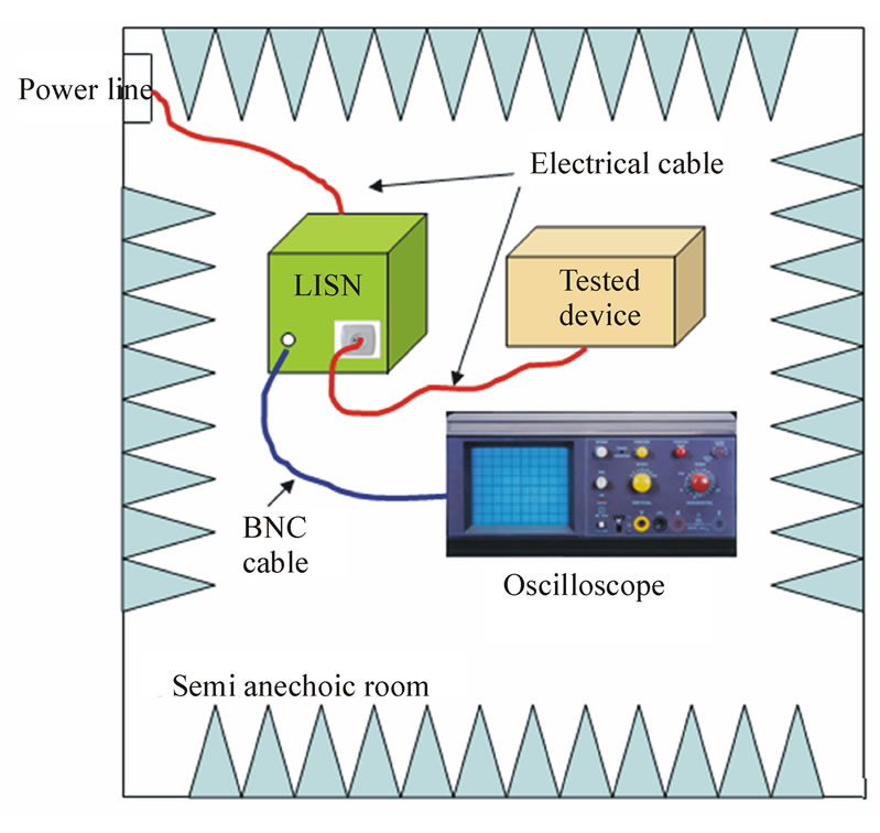
Figure 1. Measurement hardware of impulsive noise at source.
- Class 2: Electrical switch and thermostat OFF event.
- Class 3: Electrical plug plugging.
- Class 4: Electrical plug unplugging.
- Class 5: Electrical motor start.
- Class 6: Diverse weak noise signatures.
In this section, an analytical model of impulsive noise is proposed for each class. The noise model is based on the assumption that each impulse noise is a succession of elementary sub-pulses, as demonstrates, for example, on Figure 2. In Figure 3 is reported a typical sub-pulse from the impulsive noise of Figure 2.
Modeling elementary sub-pulses leads to an impulsive noise model when inter-arrival between sub-pulses and total duration models are also considered.
We proposed to model each sub-pulse by a variable-amplitude Gaussian which is phase-shifted in order to generate a set of sub-pulses that resemble as closely as possible to the measures. The noise generator reference model is reported in Figure 4.
The sub-pulses model is detailed in the Sub-Section 2.1 below. A model of sub-pulse amplitude by noise class is given. In this model, only will be excluded the class 6 because it’s composed of low-amplitude noises [1] not likely to affect the data transmission. After that, an inter-arrival between sub-pulses model, also for each noise class, is proposed in Section 2.2. And in Section 2.3 is considered the total duration of impulsive noises of each class.
In Section 2.4 is proposed a model that includes all classes at once and provides impulsive noises with the same characteristics (amplitude, duration...) than those measured. An example of a generated impulsive noise at its source by the proposed model is finally given.
2.1. Modeling of Elementary Sub-Pulses
As said above, a variable-amplitude phase-shifted Gaus-
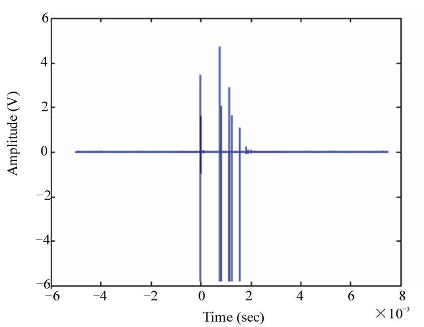
Figure 2. Coffee maker turning ON event.
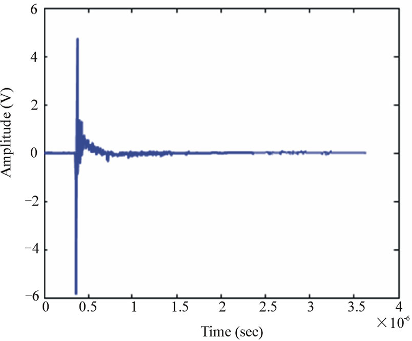
Figure 3. Sub-pulse from the impulsive noise of a coffeemaker starting ON event.
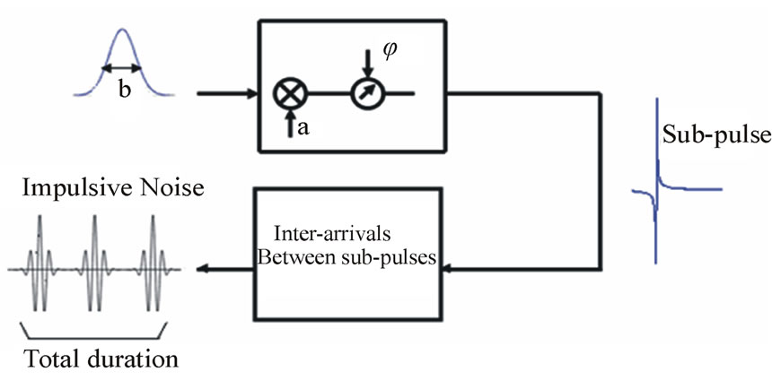
Figure 4. Reference diagram of the proposed noise model.
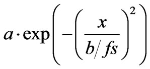
sian is proposed to model each sub-pulse. The proposed model is firstly defined by the Gaussian:
 (1)
(1)
where x is the time in seconds, and fs is the sampling frequency in Hz.
This Gaussian is two-parameter dependant: the Gaussian amplitude a and the Gaussian width represented by the b parameter. b is divided by the sampling frequency fs in order to keep generating Gaussians with representative widths when fs changes.
In order to resemble as closely as possible to the measures, this Gaussian is phase-shifted randomly by . In Figure 5 are given two phase-shifted Gaussians by
 (in blue) and
  (in red). For sake of readability, in these two figures the mean value of the Gaussians is offset from 0.
In Figure 6 are shown respectively the measured sub-pulse of Figure 3 and the generated sub-pulse according the model above. In this example a was fixed to
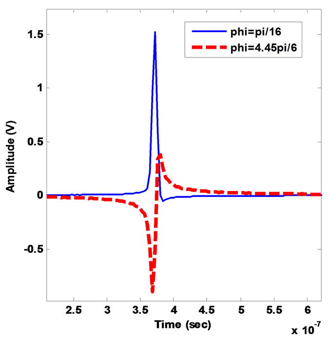
Figure 5.Phase-shifted Gaussian  (blue) and
  =
=  (in red).
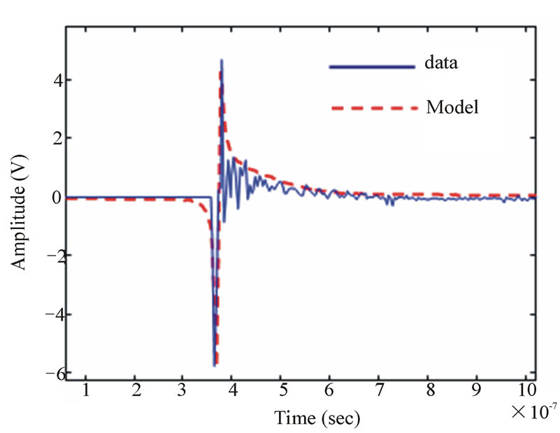
Figure 6. Sub-pulse modelling example.
8.6 V and the phase shift φ to . We note a good agreement between the measured sub-pulse and the proposed model.
We note also that the proposed model does not follow the small oscillations of the measured sub-pulse. To improve its accuracy and better fit these oscillations, a more complex GPOF model [20] will be considered in a future paper.
2.1.1. Amplitudes Modeling of Sub-Pulses
In order to model the amplitudes of sub-pulses (a in Equation (1)), these values are extracted from all subpulses of the measured noises. Then the Probability Density Function (PDF) of their absolute values is calculated for each class. An exponential distribution was finally chosen to fit the calculated PDFs. This distribution is given by:
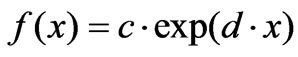 (2)
(2)
where  is the amplitude in Volts.
In Figure 7 are given the PDF results for the subpulses amplitudes of the class 1 noises. The solid blue curve is associated to the measured amplitudes and the dashed red curve is that of the proposed model, where c = 0.83 and d = –0.29.
The parameters c and d values for all classes are reported in the Table 1 below, and reported models are shown in Figures 8, 9, 10 and 11.
2.1.2. Widths Modeling of Sub-pulse
In this section is given a model of the widths b (see Equation (1)) of the measured sub-pulses. The histogram of the widths of the measured sub-pulses from the classes 1 to 5 is given in Figure 12.
The value of b is practically the same for all subpulses of all classes and it is fixed to 0.028 us.
2.1.3. Phase-Shifts Modeling of Sub-Pulses
The measured phase-shifts  applied to the model of Equation (1) in order to fit the measured sub-pulses of the classes 1 to 5 are given in the histogram of Figure13.
We note that  takes roughly random values between
  and
and . In our model the phase shifts will be randomly distributed in the
 interval, for all the noise classes.
2.2. Inter Arrival between Sub-Pulses
After modeling the sub-pulses, we propose, in this section, a model for the inter-arrivals between sub-pulses for the classes 1 to 5.
As done for the amplitudes, the PDFs of the measured
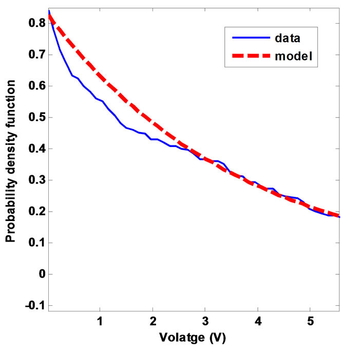
Figure 7. PDF of the amplitudes of the sub-pulses of the class 1 noises: measures (blue) vs model (red).
inter-arrivals between sub-pulses are calculated for the 5 classes, and an exponential distribution was chosen as a model:
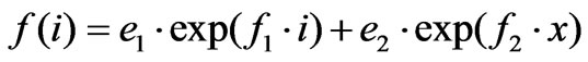 (3)
(3)
where i is the inter-arrival time in secondsIn Figure 14 are given the PDF results for the inter-arrivals between sub-pulses of the class 1 noises. The solid blue curve is the PDF of the measured inter-arrivals and the dashed red curve is that of the proposed model, where e1 = 0.6269, e2 = 0.526, f1 = –1.243E + 05 and f2 = –5626. We note that, the measured inter-arrivals between the sub-pulses of this class are comprised between 0.0019 ms and 5.5149 ms.
Equation (3) e1, e2, f1 and f2 values for the rest of classes are reported in the Table 2 below.
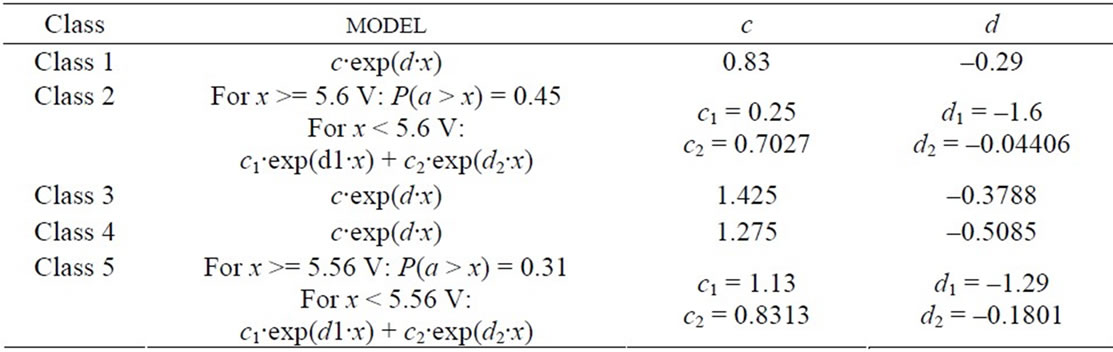
Table 1. Amplitude s of sub-pulses statistics.
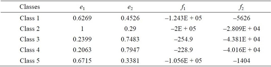
Table 2. Inter-arrival between sub-pulses statistics.
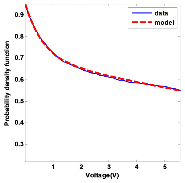
Figure 8. PDF of the amplitudes of the sub-pulses of the class 2 noises: measures (blue) vs model (red).
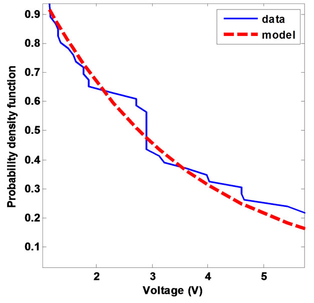
Figure 9. PDF of the amplitudes of the sub-pulses of the class 3 noises: measures (blue) vs model (red).
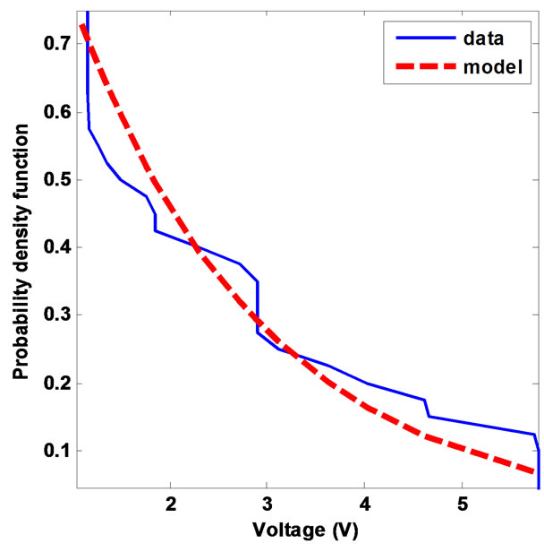
Figure 10. PDF of the amplitudes of the sub-pulses of the class 4 noises: measures (blue) vs model (red).
2.3. Total Durations Modeling of Impulsive Noises
In this section are considered the total durations of the
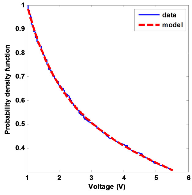
Figure 11. PDF of the amplitudes of the sub-pulses of the class 5 noises: measures (blue) vs model (red).
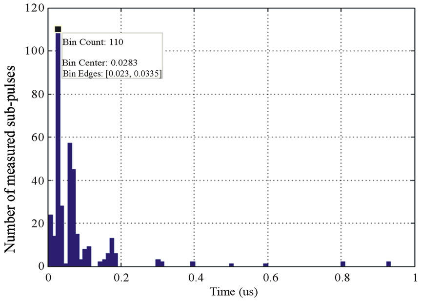
Figure 12. Histogram of the widths of the measured subpulses for the classes 1 to 5.
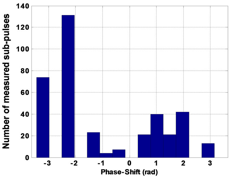
Figure 13. Histogram of phase-shifts  of the measured subpulses for the classes 1 to 5.
impulsive noises. This duration is defined as the global time since its first moment of appearance until its last time of occurrence.
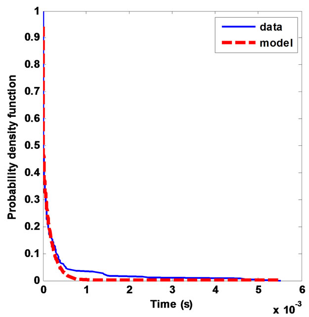
Figure 14. PDF of the inter-arrivals between sub-pulses of the class1 noises.
The curves of Figure 15 show the PDFs of the measured total durations for the noises of the classes 1 to 5.
To model such distributions, an exponential model is proposed for the classes 1 to 4:
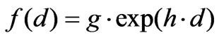 (4)
(4)
where d is the total duration in seconds. g and h parameters are given in the Table 3. And reported models are shown in Figures 16, 17, 18 and 19.
For the class 5, the distribution is modeled by the simple linear function:
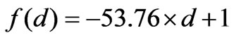 (5)
(5)
2.4. Global Impulsive Noise Model for All Classes
With a view of achieving a global noise generator for PLC channel that will help designers of communication systems on this medium to better optimize their transmission parameters, a model that includes all classes at once and provides impulsive noises with the same characteristics (amplitude, duration...) than those measured is of a great importance.
For the global impulsive noise model, we kept the same mathematical amplitude, inter-arrival between subpulses, and total duration models than those of each class. All measured amplitudes, inter arrivals and total durations are gathered together and new model parameters are calculated.
In the Figures 20, 21 and 22 are respectively given the PDF results for the sub-pulses amplitudes, inter-arrival between sub-pulses, and impulsive noises total durations for all the measured noises.
In Figure 20, given for a < 5.74 V, c1, c2, d1, and d2 parameters are respectively fixed to 2.283, 0.7296, –1.957, and –0.07138. For a ≥ 5.74 V P(a > x) is fixed to 0.4847.
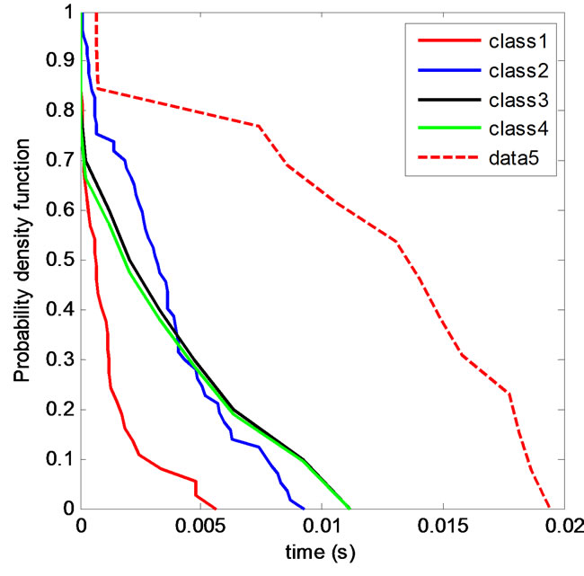
Figure 15. Total durations PDFs of the classes 1 to 5 noises.
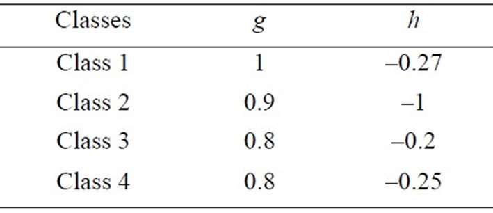
Table 3. Total durations statistics of impulse noises.
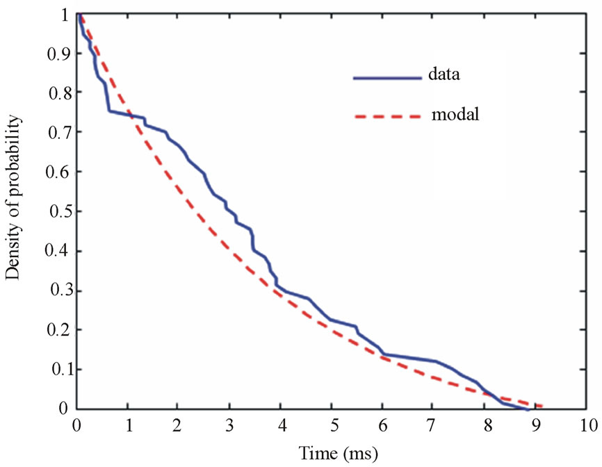
Figure 16. PDF of the total duration of the class 1 noises.
In Figure 21, the proposed model of inter-arrivals between sub-pulses given in Equation (3) is now characterized by e1 = 1.011, e2 = 0.2729, f1 = –2.407E + 05, and f2 = –1.245E + 04.
And in Figure 22, g and h parameters of Equation (4) are respectively equal to 0.5 and –0.19.
An example of generated impulse noise according to the global PDF models proposed above is given in Figure 23.
Finally, in order to model scenarios of occurrence of impulsive noise over a broad time scale, we propose in
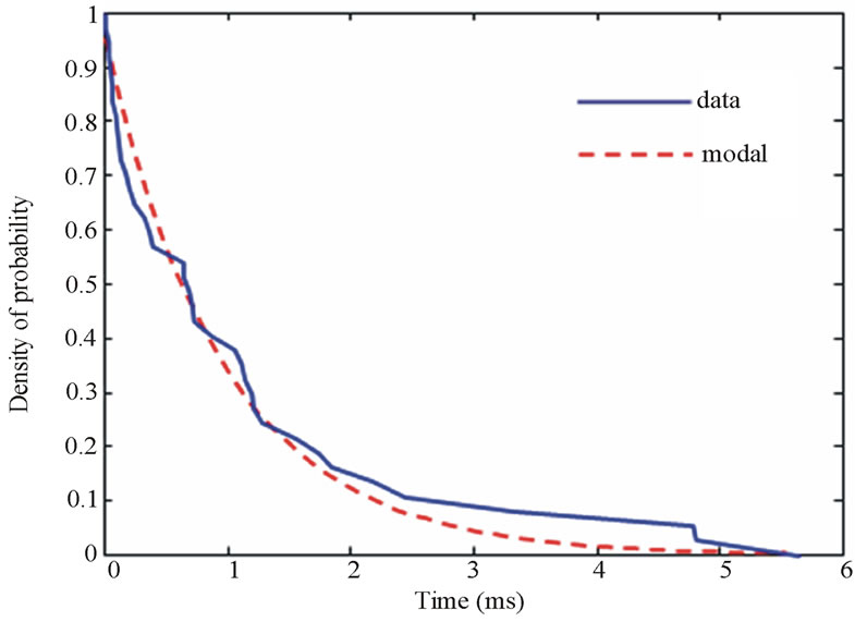
Figure 17. PDF of the total duration of the class 2 noises.
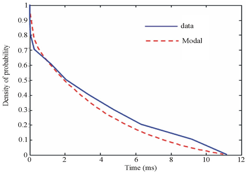
Figure 18. PDF of the total duration of the class 3 noises.
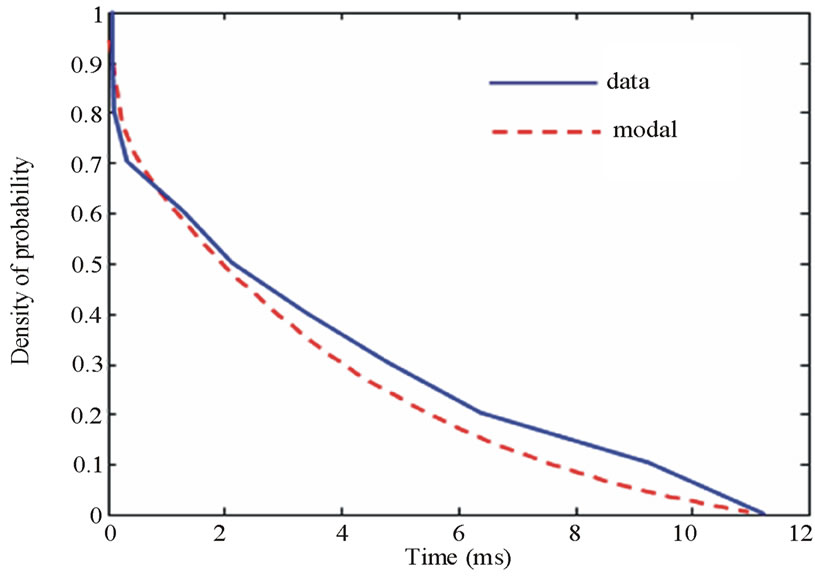
Figure 19. PDF of the total duration of the class 4 noises.
the next section a model of inter-arrivals between impulse noises. This model can be considered to quantify the damage generated by PLC impulse noise on data transmission. These quantifications can be performed over periods of 24 hours for example, and this in terms of seconds of “pixelized” video streams, number of erroneous frames.
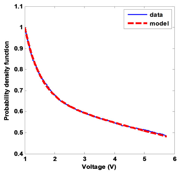
Figure 20. Global amplitudes P(a > x) model.

Figure 21. Global inter-arrivals between sub-pulses P(I > x).
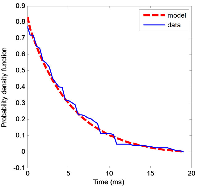
Figure 22. Global total durations P(d > x) model.
3. Modeling of Inter-Arrivals between Impulsive Noises
A second set of impulse noise measurements was carried out in several homes in order to make statistics of inter-arrivals between successive noises. Inter-arrivals between impulsive noises correspond in fact to the time
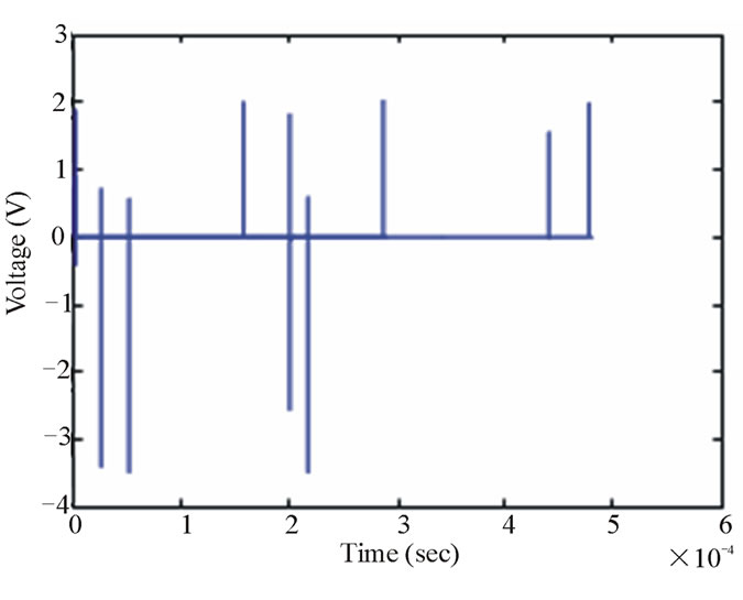
Figure 23. Generated impulsive noise—total duration = 0.48 ms.
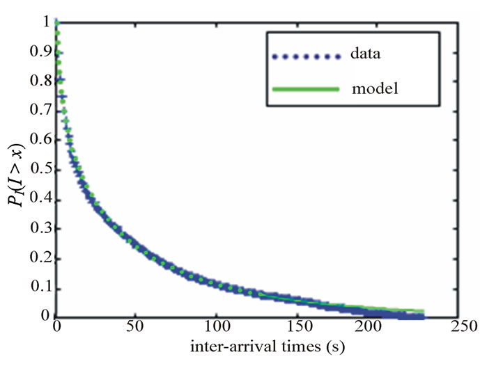
Figure 24. PI(I > x) as a function of x, where x [1 154] seconds.
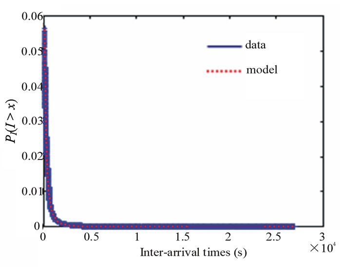
Figure 25. PI(I > x) as a function of x, where x > 154 seconds.
duration between two successive triggering events on the oscilloscope used for the measurements. The total number of measured impulsive noises was equal to 7700.
For all x > 0, we denote PI(I > x), the PDF defined by the probability that the inter-arrival I between two successive impulsive noises is greater than x seconds.
The calculated values of PI(I > x) are modelled by the Weibull distribution:
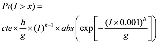 (6)
(6)
Due to the wide range of the inter-arrival values (from 1 to 2.69e4 seconds), P(I > x) is modeled in two separate intervals:
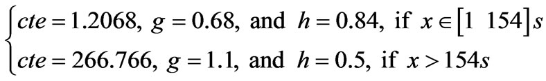
In Figures 24 and 25 are reported, for 7700 measured noises, the PI(I > x) values calculated from the data and model for both intervals.
We note a good agreement between measured PI(I > x) values and the proposed model.
4. Conclusions
In this paper, an innovative modelling approach is applied to impulsive noise which is studied directly at its source. Measuring impulsive noise at the source led us to analyse much less noises compared to noise measurements at the receiver side. Such approach permitted also to establish a correlation between the noise signature and the effective in-device noise generators: electrical switches, thermostats, electrical plugs, and electrical engines.
Based on observations we done on the measures, impulsive noises were classified into 6 different classes.
A new analytical model is proposed for each noise class. In this model each impulsive noise at source is described by a succession of short sub-pulses, each modeled by a variable-amplitude phase-shifted Gaussian. To generate impulsive noises, distributions of the inter-arrivals between sub-pulses and total noise durations were also considered for each class.
A noise model that included all classes at once was also given. And so that we can model scenarios of occurrence of impulsive noise over a broad time scale, a model of inter-arrivals between impulse noises was finally proposed.
As mentioned in the amplitude description section, the proposed model does not follow the small oscillations of the measured sub-pulses. To improve its accuracy and better fit these oscillations, a more complex GPOF model [19] will be considered in a future paper.
REFERENCES
- M. Tlich, H. Chaouche, A. Zeddam and P. Pagani, “Novel Approach for PLC Impulsive Noise Modelling,” IEEE International Symposium on Power Line Communications and Its Applications, Dresden, 29 March-1 April 2009, pp. 20-25.
- K. Dostert, “Telecommunications over Power Distribution Grid: Possibilities and Limitations,” International Symposium on Power-Line Communications and Its Applications, Essen, 2-4 April 1997.
- M. Zimmermann and K. Dostert, “A multi-Path signal propagation model for the powerline channel in the high frequency range,” International Symposium on PowerLine Communications and Its Applications, Lancaster, 30 March-1 April 1999, pp. 45-51.
- T. Esmailian, P. G. Gulak and F. R. Kschischang, “A Discrete Multitone Power Line Communications System,” Proceedings of the Acoustics, Speech, and Signal Processing, Vol. 5, Istanbul, 5-9 June 2000, pp. 2953-2956.
- E. Liu, Y. Gao, G. Samdani, Omar Mukhtar and T. Korhonen, “Broadband Power-Line Channel and Capacity Analysis,” International Symposium on Power-Line Communications and Its Applications, Vancouver, 6-8 April 2005, pp. 7-11.
- H. Meng and S. Chen, “Modeling of Transfer Characteristics for the Broadband Power Line Communication Channel,” IEEE Transactions on Power Delivery, Vol. 19, No. 3, 2004, pp. 529-551. doi:10.1109/TPWRD.2004.824430
- M. Zimmermann and K. Dostert, “A Multi-Path Model for the Power Line Channel,” IEEE Transactions on Communications, Vol. 50, No. 4, 2002, pp. 553-559. doi:10.1109/26.996069
- H. Philipps, “Development of a Statistical Model for Power Line Communications Channels,” International Symposium on Power-Line Communications and Its Applications, Limerick, 5-7 April 2000, pp. 153-160.
- D. Anastasiadou and T. Antonakoupoulos, “Multipath Characterization of Indoor Power-Line Networks,” IEEE Transactions on Power Delivery, Vol. 20, No. 1, 2005, pp. 90-99. doi:10.1109/TPWRD.2004.832373
- P. Amirshahi and M. Kavehrad, “Transmission Channel Model and Capacity of Overhead Multi-Conductor Medium-Voltage Powerlines for Broadband Communications,” International Symposium on Power-Line Communications and Its Applications, Zaragoza, 31 March-2 April 2004, pp. 354-358.
- A. Rennane, C. Konate and M. Machmoum, “A Simplified Deterministic Approach to Accurate Modeling of Transfer Function for the Broadband Power Line Communication,” INTECH, Morn Hill, 2010, pp. 1-18.
- H. Heng, S. Chen, Y. L. Guan and C. L. Law, “Modeling of Transfer Characteristics of the Broadband Power Line Communication Channel,” IEEE Transactions on Power Delivery, Vol. 19, No. 3, 2004, pp. 1057-1064. doi:10.1109/TPWRD.2004.824430
- M. Tlich, A. Zeddam, F. Moulin, F. Gauthier and G. Avril, “A Boadband Powerline Channel Generator,” Proceedings of the IEEE International Conference on Power Line Communications and Its Applications, Pisa, 26-28 March 2007, pp. 505-510.
- M. Tlich, A. Zeddam, F. Moulin and F. Gauthier, “Indoor Power-Line Communications Channel Characterization up to 100 MHz. Part I: One-Parameter Deterministic Model,” IEEE Transactions on Power Delivery, Vol. 23, No. 3, 2008, pp. 1392-1401. doi:10.1109/TPWRD.2008.919397
- G. Avril, M. Tlich, F. Moulin, A. Zeddam and F. Nouvel, “Time/Frequency Analysis of Impulsive Noise on Powerline Channels,” 1st International Home Networking Conference, Paris, 10-12 December 2007, pp. 143-150.
- M. Zimmermann and K. Dostert, “An Analysis of the Broadband Noise Scenario in Power-Line Networks,” International Symposium on Power-Line Communications and Its Applications, Limerick, 5-7 April 2000, pp. 131-138.
- V. B. Balakirsky and A. J. H. Vinck, “Potential Limits on Powerline Communication over Impulsive Noise Channels,” International Symposium on Power-Line Communications and Its Applications, Kyoto, 26-28 March 2003, pp. 32-36.
- V. Degardin, M. Lienard, P. Degauque, A. Zeddam and F. Gauthier, “Impulsive Noise on Indoor Power Lines: Characterization and Mitigation of Its Effect on PLC Systems,” IEEE International Symposium on Electromagnetic Compatibility, Vol. 1, Istanbul, 11-16 May 2003, pp. 166-169.
- F. Rouissi, “Optimisation de la Couche Physique des systèmes de communication sur le réseau d’énergie en présence de bruit Impulsif,” Thesis, Lille, May 2008.
- H. Chaouche, A. Zeddam, F. Gauthier, M. Tlich and M. Machmoum, “Mesure et Modelisation du Bruit Impulsif à la Source,” 15ème Colloque International et Exposition sur la Compatibilité Électromagnétiqu, Limoges, 7-9 April 2010, pp. 3-4.