Int'l J. of Communications, Network and System Sciences
Vol. 5 No. 4 (2012) , Article ID: 18520 , 5 pages DOI:10.4236/ijcns.2012.54027
Extending Instrumental Variable Method for Effective Economic Modelling*
1School of Economic and Management, Dalian Nationalities University, Dalian, China
2Department of Economics and Management, Northeastern University in Qinhuangdao, Qinhuangdao, China
Email: zhengshi1993@yahoo.com.cn
Received December 20, 2011; revised January 29, 2012; accepted February 13, 2012
Keywords: ARX modeling; Parametric Estimation; Instrumental Variable Method; Northeastern Economy; Exogenous Variables
ABSTRACT
Economic modeling that yields practical value must cater for effects caused by exogenous variables. AutoRegressive eXogenous approach (ARX) has been widely used in regional economic studies. Instrumental Variable Method is regarded as a preferential method to parametric estimation in ARX modeling. However, traditional instrumental variable methods can only handle single variable which has limited its capability. This paper presents an extended instrumental variable method (EIVM) which is based on multiple variables. This provides the capability of taking into account of exogenous variables and reflects better the economic activities. A case study is conducted, which illustrates the application of the EIVM in modeling Northeastern economy in China.
1. Introduction
Economic modeling that yields practical value must cater for effects caused by exogenous variables. Many linear models such as time series, regression and econometric models can describe the relationship between system inputs and outputs. However, such systems reflect the simple relationship between cause and effect, therefore are the result of Newtonian mechanical causation theory. Autoregressive eXogenous approach (ARX) has been widely used in regional economic studies so as to tackle this problem. Instrumental Variable Method is regarded as a preferential method to parametric estimation in ARX modeling.
For more than 40 decades, scholars all over the world focus on regional economic strategies. The policy measurements and regional economic administration methodology are often discussed. However, the research on them is still lagged behind the management theory study. For instance, there are 10000 pieces of papers about the theory innovation of the regional economic administration from 2003 to 2010, besides thse 16 pieces of papers from the journal indexed by EI. There are few mature regional economic models, including CAS model [1], changing CAS model [1], and CGE model [2,3] etc.
Too many variables were placed in these models so that they are more complex and the control strategies on basis of them are also complicated. For the aforementioned reasons, some experts believe that the quantities administration of the regional economic system can not work. Fortunately, ARX models were employed in regional economic administration in 2007 [4,5]. It is a progress in the quantities administration of the regional economic system because the model has sufficient information and the structure of the model is simple. Nevertheless, the estimation process of the MIMO ARX model in detail had not been mentioned by the prior researches.
Our aim is to present an extended instrumental variable method (EIVM) which is based on multiple variables. This provides the capability of taking into account of exogenous variables and reflects better the economic activities. A case study is conducted, which illustrates the application of the EIVM in modeling Northeastern economy in China.
2. Extending Instrumental Variable Method
In this section, MIMO ARX parametric model is constructed and Extending Instrumental Variable Method is proposed.
2.1. MIMO ARX Parametric Model
Parametric models are a family of mathematical models, in forms such as difference equations, differential equations, state-space equations, and auto regressive model. Among the auto regressive models, the ARX parametric model is more accurate one to describe the exogenous variables, such as macro policies, regional policies.
The MIMO ARX model is constructed as follows:
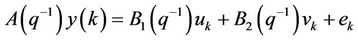 (1)
(1)
where  is the unit lag operator,
  ,
,  ,
,  are the parameters of the MIMO ARX model (1), i.e. lagged operator or translation operator polynomial.
  is a random error term.
2.2. Parameter Optimization
The traditional parameter optimization process of the ARX model includes estimation of the parameters and order selection of the model. The parameter optimization process of MIMO ARX parametric model is similar as it.
2.2.1. Estimation of the Parameters
Parametric estimation is the process to estimate the parameters of the ARX model by an error criterion. The mature methods are least square method [6] and improved least square method [7]. Other methods include error prediction estimation method [8], IV estimation method [9] and the mathematical approximation method, such as the forward-backward method [10], Yule-Walker method, Burg method [11], the geometric lattice method [12]. Among them, IV estimation method is simple at some extent, and it can be used under many circumstances [13].The unbiased estimation value can be obtained, when the residuals are auto-regression [14,15]. The inputs signals are disturbed by the white noises. Because the statistical indices collected are influenced by all kinds of errors. For the input terminal perturbation, input error criteria can be used [16]. However, the system identification algorithm is more complex since the input error is related to the nonlinear function of the model parameters. Gao & Xu [17] proposes that the inputs noises can be transformed into outputs noises in an ARMA parametric model. In this way, the white noises of inputs terminal can be regarded as colored noises of outputs terminal. It can be proved that the aforementioned statement is also valid in a MIMO ARX parametric model. Since the optimization process of the parameters in an ARX model is similar of that in an ARMA model. Thus, equation (1) is transformed as follows:
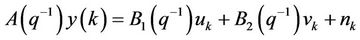 (2)
(2)
where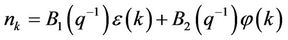 .
.
The local linear equation can be rewritten as:
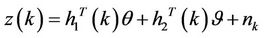 (3)
(3)
where


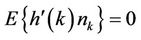
After the selection of the model order, instrumental variables can be taken as a random vector  which has the same distribution and independent with the inputs signals according to
  principle. Since the inputs signals are unrelated with the errors
 , we can obtained,
For the  in k’s domain,

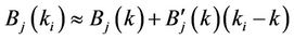
where  depicts derivative of degree 1 of
 . Then for any given value
 , the local instrumental variable estimation
  of
of  is defined as the solution of the following simultaneous equations:
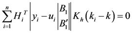 (4)
(4)
 (5)
(5)
where,  ,
,  ,
,  is the
  line of the following matrices
 ,
,  ,
,  ,
,
 .
.
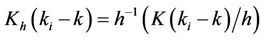
 is named as kernel function (i.e. weight function),
  ,
,  depicts window width, it determine the size of the local domain.
Furthermore, the local linear estimation overcomes the shortcomings of the normal kernel estimation. The convergence rate of estimation error at the boundary points is lower than that at the interior point of the latter. Thus, special kernel function can not be taken in the local linear estimation.
2.2.2. The Selection of the Model Order
For the MISO linear difference equations model, since the system noises are colored noises, the IV estimation method can be employed in order to obtain unbiased estimation of the model parameters. Because the identification of the model order is also needed, the order search method should be used. Increasing the model order successively, Estimating the model parameters and the loss function value under different model order, then taking advantaging the loss function value, the model order can be determined by the AIC criteria.
3. Case Study
In this section, a case study for the northeastern economy is conducted.
3.1. Data Collection and Model Construction
The Prediction and dynamically control of the northeastern economy in China is a major aim for Chinese regional administration. The nonlinear characteristics dynamics of the process depend on the output of the northeastern economy. The observable nonlinear characteristics are sourced from the fluctuation of the competitiveness. There was considerable time delay involved in the competitiveness indices (for instance, a macropolicy or regional policy released in seven years ago brings about policy effect in this year). We took Liaoning province as a case; the structure of model (1) was employed. On the basis of 6 years statistical data (2000-2005), the system identification method in Matlab toolbox was extended and applied to the system identification of the model (6).
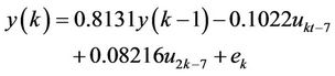 (6)
(6)
Model (6) is a mature regional economic model in literature [3], where the noises are colored one.
3.2. Package of EIVM
Since there is no method can estimate MIMO ARX model in Matlab Toolbox, an estimation program of EIVM is designed.
There are four parameters of EIVM, i.e. z, nn, adm, adg. The fomular can be written by
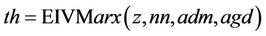 (7)
(7)
 , nn depicts the modle order, adm and adg depicts the type of recursive least squares algorithm.
In order to realize identification on-line and reduce the memory occupation, recursive estimation method was employed. There are different kinds of recursive methods, such as many transformation of estimation method offline, Kalman Filter method, stochastic approximation method, model reference adaptive parameters recursive estimation method. The extended instrumental variable method and recursive estimation are employed. The formula is as follows:
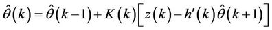 (8)
(8)
The estimation process in detail is as follows:
1) 400 impulse sequence signals is generated as input.
2) Gaussian white noise which mean is equal to 0 and variance is equal to 1 is generated.
3) Input observation sequence.
4) Recursive estimate.
a) variance estimate.
b) store estimation value in intermediate process.
c) Construct the augmented matrix.
d) Construct instrumental variables.
e) Calculate K value.
f) Estimate the final th.
After programming and calculating, the following model was obtained:
 (9)
(9)
The model fitness is 89.25. The loss function is 0.000776957. The FPE (Final Predictive Error) is 0.00129493.
3.3. Simulations
3.3.1. Simulations Environment and Parameters
Matlab is a powerful simulation tool; it was employed in the empirical study in this paper. Command “idsim” is adopted.
Since is recursive method based on Kalman Filter method is designed in EIVM. adm, adg are ignored. z, nn, should be considered as parameters.
3.3.2. Simulations Process
In order to make the process simplified and concise, the model order is default by [1 1 7] according to model (6). Simulation program Inventory is as follows:
% clear A = [1 − 0.8131]
B = [B0,B1,B2,B3,B4,B5,B6,B7]
B0 = [0 0]
B1 = [0 0]
B2 = [0 0]
B3 = [0 0]
B4 = [0 0]
B5 = [0 0]
B6 = [0 0]
B7 = [−0.1022 008216]
u1 = [0.09758 0.0849 0.0413 0.01413 0.106 0.0457]
u2 = [0.0103 0.008889 0.0117 0.00889 0.0117 0.0117]1
th0 = arx2th (A,B,1,2)
e = rand (200,1)
u = [u1 u2]
y = idsim([u e],th0)
z = [y u]
th = eivm(z, [1 1 7])
plot(y,’-‘)
hold on Figures 1 and 2 show the transition process of the parameters and variance to be estimated. From the two figures, we can find the convergence rate in the 400 observable time series is closed to 0 in a short period. That means the method is valid in practice. Comparing with the LSM, IV or other estimation method of system identification toolbox in Matlab software package, the error message would be given. For example, when LSM is employed, a tip is given to increase the ample size or reduce the model order in Matlab workspace. While other nonlinear parametric estimation methods were tried, the module tips show that too many parameters to be estimated, thus no result was given.
We also applied EIVM in identifying the ARX parametric models of Jinlin and LiaoNing province; we omitted it in this paper.
In sum, we attempt by various methods and find the extended instrumental variable method is valid in northeastern economy identification. It can be applied to other areas for the system identification.
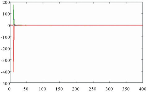
Figure 1. The transition process of the parameters to be estimated.
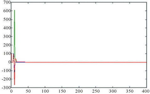
Figure 2. The transition process of the variance to be estimated.
4. Conclusions
The method proposed in this paper is an extension of the method in [17] and [18]. The method in this paper not only has a high convergence rate but also abroad application prospect for the situation which other methods cannot work. It has advantages for the nonlinear systems such as a regional economic system etc. It also has important value in practice, when it was applied to the system with large time delay. Therefore, it has great strategic significance in tackling the extensive management problem which occurred in the northern-east economy, as well as in improving the management efficiency.
The future work should focus on the application of EIVM as well as the hybrid of the method with other methods such as mentioned in [19-21].
REFERENCES
- Z. H. Zhu, “A Primary Study of Regional Economic System Model,” Journal of Systemic Dialectics, Vol. 7, 2005, pp. 74-77.
- M. D. Partridge and D. S. Rickman, “Computable General Equilibrium (CGE) Modelling for Regional Economic Development Analysis,” Regional Studies, Vol. 12, No. 10, 2010, pp. 1311-1328. doi:10.1080/00343400701654236
- D. S. Rickman, “Modern Macroeconomics and Regional Economic Modelling,” Journal of Regional Science, Vol. 50, No. 1, 2010, pp. 23-41. doi:10.1111/j.1467-9787.2009.00647.x
- S. Zheng, W. Zheng and X. Jin, “Estimation of ARX Parametric Model in Regional Economic System,” Systems Engineering, Vol. 10, No. 4, 2007, pp. 290-296. doi:10.1002/sys.20077
- S. Zheng, W. Zheng and X. Jin, “Fuzzy Integration Monitor Method in Regional Economic System and Its Simulation,” 26th Chinese Control Conference, Hunan, 23-31 July 2007, pp. 2-4.
- Y. G. Li, M. F. A. Ghafir and L. Wang, “Improved Multiple Point Nonlinear Genetic Algorithm Based Performance Adaptation Using Least Square Method,” Journal of Engineering for Gas Turbines and Power, Vol. 134, No. 3, 2012, p. 031701. doi:10.1115/1.4004395
- T. Oztekin, “Estimation of the Parameters of Wakeby Distribution by a Numerical Least Squares Method and Applying It to the Annual Peak Flows of Turkish Rivers,” Water Resources Management, Vol. 25, No. 5, 2011, pp. 1299-1313. doi:10.1007/s11269-010-9745-2
- M. Arif, T. Ishihara and H. Inooka, “Iterative Learning Control Utilizing the Error Prediction Method,” Journal of Intelligent and Robotic Systems, Vol. 25, No. 2, 1999, pp. 95-108. doi:10.1023/A:1008099704692
- M. Cedervall and P. Stoica, “System Identification from Noisy Measurements by Using Instrumental Variables and Subspace Fitting,” Circuits, Systems, and Signal Processing, Vol. 15, No. 2, 1996, pp. 275-290. doi:10.1007/BF01183780
- S. Haubruge, V. H. Nguyen and J. J. Strodior, “Convergence Analysis and Applications of the Glowinski-Le Tallec Splitting Method for Finding a Zero of the Sum of Two Maximal Monotone Operators,” Journal of Optimization Theory and Applications, Vol. 97, No. 3, 1998, pp. 645-673. doi:10.1023/A:1022646327085
- A. Subasil, “Application of Classical and Model-Based Spectral Methods to Describe the State of Alertness in EEG,” Journal of Medical Systems, Vol. 29, No. 5, 2005, pp. 473-486. doi:10.1007/s10916-005-6104-6
- K. L. Nyman, “Linear Inequalities for Rank 3 Geometric Lattices,” Discrete Computational Geometry, Vol. 31, No. 2, 2004, pp. 229-242. doi:10.1007/s00454-003-0807-6
- Z. Zheng and S. Tian, “Supplementary Variable Parameter Identification and Emulate Based on Matlab,” Computer Application and Software, Vol. 21, No. 7, 2004, pp. 127-129.
- X. L. Wang and W. J. Ji, “Refined-Optimal Instrumental Variable Algorithm and Its Simulation,” Control Theory and Applications, 1989, pp. 100-105.
- L.-Y. Wei, C.-H. Cheng and H.-H. Wu, “Fusion ANFIS Model Based on AR for Forecasting EPS of Leading Industries,” International Journal of Innovative Computing, Information and Control, Vol. 9, No. 7, 2011, pp. 5445- 5458.
- B. Chen, “The Application of Instrumental Variable Method in the Estimation of Parameters of ARMA(p,q) Model,” Journal of Xuzhou Normal University (Natural Science Edition), Vol. 12, 1990, pp. 31-37.
- H. L. Gao and B. L. Xu, “The Application of IV Method and Its Improved Algorithm to Noisy System Parameter Estimation,” Journal of Nanjing University (Natural Sciences), Vol. 1, 1977, pp. 27-31.
- Y. Sun, “Theory and Method of Estimation for Varying Coefficient Macroeconomics Simultaneous Equations Model,” Mathematics in Practice and Theory, Vol. 3, No. 4, 2009, pp. 60-66.
- O. Rizal and Z. Zhang, “Takashi Imamura and Tetsuo - Miyake. Driver Inattention Analysis Using Neural Network Based Nonlinear ARX Model,” ICIC Express Letters, Part B: Applications, Vol. 2, No. 3, 2011, pp. 679-686.
- J. G. Weber and N. Key, “How Much Do Decoupled Payments Affect Production? An Instrumental Variable Approach with Panel Data,” American Journal of Agricultural Economics, Vol. 94, No. 1, 2012, pp. 52-66. doi:10.1093/ajae/aar134
- X. J. Yan, et al., “Parametric System Identification Based on Instrumental Variable Method,” Machine Tool & Hydraulics, Vol. 12, 2006, pp. 181-182.
NOTES
*This research is supported by Liaoning Social Science funds (Project No. L07DJY067) and Ph.D. support funds (20066201). Also supported by the “Fundamental Research Funds for the Central Universities” (Project No. DC10030207) and DaLian S&T Bureau Funds (Project No. 2011J21DW020).
1Sourced from results of project of Liaoning department of Education (Project No. 05w028), u1 depicts core-element competitiveness u2 depicts Auxiliary-element competitiveness.