Journal of Water Resource and Protection
Vol.6 No.11(2014), Article
ID:48704,11
pages
DOI:10.4236/jwarp.2014.611091
Analysis of Water Stress Prediction Quality as Influenced by the Number and Placement of Temporal Soil-Water Monitoring Sites
Luan Pan1, Viacheslav I. Adamchuk1*, Richard B. Ferguson2, Pierre R. L. Dutilleul3, Shiv O. Prasher1
1Department of Bioresource Engineering, McGill University, Ste-Anne-de-Bellevue, Canada
2Department of Agronomy and Horticulture, University of Nebraska-Lincoln, Lincoln, USA
3Department of Plant Science, McGill University, Ste-Anne-de-Bellevue, Canada
Email: *viacheslav.adamchuk@mcgill.ca
Copyright © 2014 by authors and Scientific Research Publishing Inc.
This work is licensed under the Creative Commons Attribution International License (CC BY).
http://creativecommons.org/licenses/by/4.0/


Received 20 June 2014; revised 16 July 2014; accepted 2 August 2014
ABSTRACT
In an agricultural field, monitoring the temporal changes in soil conditions can be as important as understanding spatial heterogeneity when it comes to determining the locally-optimized application rates of key agricultural inputs. For example, the monitoring of soil water content is needed to decide on the amount and timing of irrigation. On-the-go soil sensing technology provides a way to rapidly obtain high-resolution, multiple data layers to reveal soil spatial variability, at a relatively low cost. To take advantage of this information, it is important to define the locations, which represent diversified field conditions, in terms of their potential to store and release soil water. Choosing the proper locations and the number of soil monitoring sites is not straightforward. In this project, sensor-based maps of soil apparent electrical conductivity and field elevation were produced for seven agricultural fields in Nebraska, USA. In one of these fields, an eight-node wireless sensor network was used to establish real-time relationships between these maps and the Water Stress Potential (WSP) estimated using soil matric potential measurements. The results were used to model hypothetical WSP maps in the remaining fields. Different placement schemes for temporal soil monitoring sites were evaluated in terms of their ability to predict the hypothetical WSP maps with a different range and magnitude of spatial variability. When a large number of monitoring sites were used, it was shown that the probability for uncertain model predictions was relatively low regardless of the site selection strategy. However, a small number of monitoring sites may be used to reveal the underlying relationship only if these locations are chosen carefully.
Keywords:On-the-Go Soil Sensing, Variable-Rate Irrigation, Electrical Conductivity, Site-Specific Water Management, Soil Matric Potential

1. Introduction
When pursuing site-specific crop management, temporal variability in soil water content is frequently as important as spatial variability. Thus, in order to optimize irrigation water management, one should combine the knowledge of changes of soil water holding capacity across a field with temporal monitoring of the actual water content available to plants during the most critical phases of crop production. Implementing this “precision irrigation” strategy means optimizing both the quantity and the timing of irrigation that may vary across a field due to different soil and growing conditions. Using traditional soil analysis practices, without considering soil spatial heterogeneity, is not optimal when it comes to site-specific water management.
Proximal soil sensing technology makes it possible to obtain high-resolution maps pertaining to different soil properties at a relatively low cost [1] . Unfortunately, the relationships between the data detected on-the-go and agronomic soil parameters such as water content are frequently site-specific. In addition, the amount of water stored in the soil profile changes not only spatially, but also temporally. Therefore, sensor-based maps have been used to define the spatial variability of soil properties influencing water movement and storage across a landscape, and this information has been used to define relatively homogeneous management zones that have been evaluated separately [2] .
Increasingly, wireless technology is used to achieve temporal monitoring of soil conditions. Such systems allow the producer to obtain information about soil water content, temperature, and other properties in real-time from a remote location [3] . This technology greatly improves the convenience of monitoring soil water for the producer. Irrigation system managers have employed the data to optimize the use of resources in response to dynamic changes in soil water content and to reduce the risk of crop water stress [4] -[6] .
Selecting a number of strategic locations within the field is not trivial and is mostly subjective. Practitioners who use high-resolution data layers apply the following general rules: 1) cover the entire range of data from each source, 2) avoid field boundaries and other transition zones, and 3) spread locations over the entire field. Quality coverage of the entire data space is important to make sure that both dry and wet field locations are monitored. Boundary and transition areas are avoided to make sure monitoring locations and spatially variable field characteristics represent the same local conditions. Finally, the geographic spread is needed to account for any additional uncertainties, such as possible spatially variable amounts of rainfall.
While the criteria listed above are useful, they do not translate into an operational algorithm and, therefore, can produce numerous solutions with different degrees of satisfaction. In principle, this process is similar to prescribing targeted sampling locations to either calibrate high-resolution data, or to quantify the agronomic soil attributes of established management zones [7] -[11] . Determination of the number of target sampling locations is another critical task.
With an ultimate goal of developing an algorithm for optimization of a wireless sensor network design, the objective of this study was to quantify the influence of the number and locations of temporal soil-water monitoring sites on the quality of water stress potential predictions within a set of hypothetical fields representing different levels of spatial variability.
2. Materials and Methods
2.1. Experimental Data
Seven agricultural fields in Nebraska (Figure 1) were mapped using on-the-go sensing technology with a Veris® 3150 or 3100 unit (Veris Technologies, Inc., Salina, Kansas)1 equipped with an RTK-level global navigation satellite system (GNSS) receiver. Apparent soil electrical conductivity (ECa) and field elevation (altitude) were used to assess the spatial variability for soil water storage. In one of these fields (a 37-ha field at the Agricultural

Figure 1. Research fields in Nebraska, USA.
Research and Development Center (ARDC) near Mead, Nebraska, USA), eight locations under a center-pivot irrigator were selected for monitoring the soil matric potential and the temperature using wireless sensor technology [12] . For each location, the Water Stress Potential (WSP), originally called Water Stress Index, was calculated as:
 (1)
(1)
where wi is the weighting factor for water extracted in the plant root zone for depth increment i; Ψi is the soil matric potential measurement at the ith depth, kPa; and  is the soil-specific soil matric potential at certain threshold level of soil water depletion (25% depletion was used in this research as half of the most frequently cited percent depletion causing water stress in corn) at the ith depth, kPa.
The following regression model [12] was used to define time-specific relationships between the high-density spatial data and WSP:
 (2)
(2)
where ECa is apparent soil electrical conductivity, mS/m; Elev is field elevation, m; β0, β1, β2, β3 are model coefficients.
Since a different set of regression coefficients was established for any point in time, it was possible to generate WSP maps using each new regression model. Thus, 99 sets of regression model coefficients were determined for every day of the 2009 growing season in the ARDC field (Figure 2). July 30th, 2009 (day 33) was chosen as an example of a regression equation that linked WSP, ECa and field elevation in the middle of the growing season:
 (3)
(3)
This equation can be generalized by using relative field elevations (obtained by subtracting the median elevation) instead of the original field elevation values:
 (4)
(4)
where Elevrel is the relative field elevation.
To evaluate the quality of the WSP prediction using different distributions of temporal monitoring stations, it is important to know the WSP value in every location in the field, or at least, across a substantial number of validation locations. Unfortunately, this is not practical because of the high cost of temporal monitoring locations and numerous uncertainties at a fine scale. Therefore, an alternative analytical approach has been used in this study. Equation (4) was assumed to be valid for the other six fields (BR, HS, HU, KR, LU, and RU), which would allow modeling hypothetical maps of WSP at the same resolution as soil ECa and field elevation maps. These new fields represented diversified conditions in terms of field topography and soil heterogeneity (Table 1). In each case, both ECa and elevation data were interpolated (Inverse Distance Weighting) using a 10 × 10 grid, and corresponding maps were obtained for the calculated WSP values (Figure 3). Each of these maps is a hypothetical representation of what could be the WSP distribution across a given field at a specific time, assuming the regression equation (4) has a perfect fit.
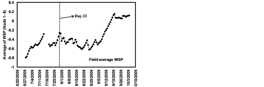
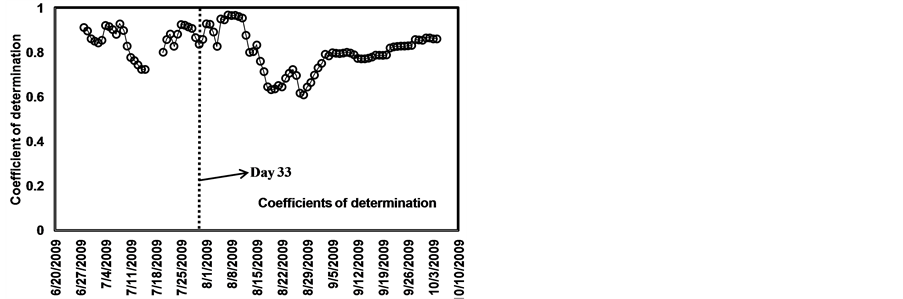

Table 1. Field description.
2.2. Error Simulation
Since in reality the regression model linking the WSP with ECa and elevation is an approximation, the actual WSP map is different from the calculated WSP. To model a WSP map that could represent the actual state-of-nature, three different error simulation strategies were used to represent different degrees of spatial structure. Table 2 summarizes the spatial structure used to simulate error surfaces. All three surfaces had the same total variance (sill = 0.04), which was similar to what had been observed in the ARDC field, and a mean error equal to zero, which was used to avoid bias between different modeled WSP maps (Figure 4). The first surface was assumed to have no spatial structure, while the second surface was simulated using an arbitrary spherical variogram model with a zero nugget effect and 300-m range of spatial dependency. The third surface was an intermediate case with a range two times smaller and a partial sill equal to the nugget effect.
Figure 5 illustrates three simulated WSP maps obtained for the HS field. Such error surfaces covering the extents of each field were superimposed on the calculated WSP maps. Then, these error surfaces were clipped to the
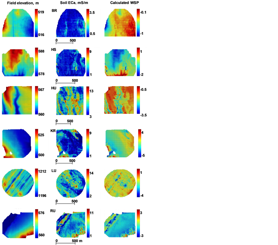
Figure 3. Maps of field elevation, soil ECa, and calculated WSP.
Table 2. Variogram parameters for three error surfaces (ES 1-3).
actual field shape and re-scaled to maintain a zero-mean error and the simulated spatial structure. Each of the resulting maps was an example of the hypothetical WSP distribution across the landscape that could have actually taken place in a given field at a specific time. Predicting these maps with the least possible error would require an optimal network of temporal monitoring stations.
2.3. Soil-Water Monitoring Site Selection
In practice, the definition of the optimum-guided sampling scheme is rather vague. There are many parameters that can quantify 1) spatial separation, 2) spread across both sets of measurements (in this case, ECa and field elevation), and 3) local homogeneity within each set of measurements. Furthermore, there are several different
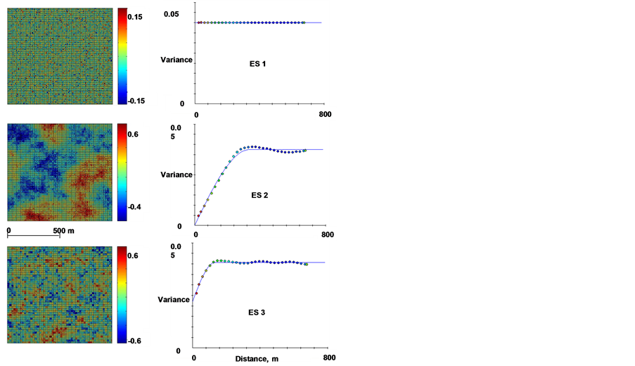
Figure 4. Maps and semivariograms of simulated error surfaces.
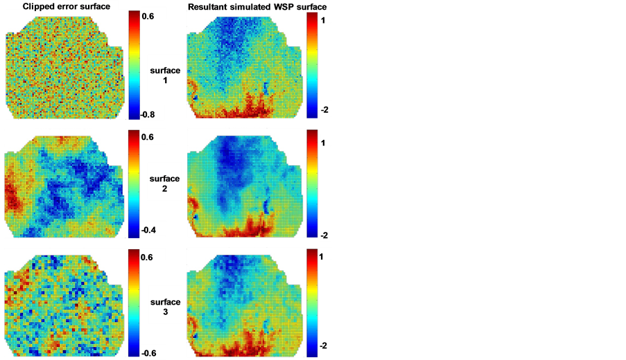
Figure 5. Maps of three simulated error surfaces clipped to the HS field shape and the resultant simulated WSP maps.
ways to derive the overall objective function as a combination of these parameters. In this study, the criteria used by Adamchuk et al. [11] were applied. These criteria included: 1) complete spatial field coverage using the S optimality criterion [13] ; 2) even distributions throughout both data layers (in this case, ECa and field elevation) using the D optimality criterion [13] ; and 3) the relative homogeneity of the selected sites using the sum of squared differences between the measurements obtained in each location and those of the nearest neighbors. While S-optimality seeks to maximize the harmonic mean distance between each monitoring location in relation to all other monitoring locations, D-optimality increases with greater coverage of the range of soil ECa and field elevation maps. The overall objective function was the geometric mean of these criteria normalized against the median of a large number of random selections. The optimized set of monitoring sites with the overall objective function closest to one was selected among 1000 randomly selected sets. In practice, the results of this optimization can be achieved through a hypercube sampling with an added requirement of geographic spread and a penalty for selecting monitoring sites in field locations with highly variable ECa or field elevation. Although alternative site section algorithms could be acceptable, typically, they rely on either design-based, or model-based, inference [9] ; in fact, both can be important.
To compare different site selection strategies, the performance of 100 randomly selected sets of soil-water monitoring sites were evaluated along with the optimally selected placements of these sites. This was repeated for each field and the number of potential soil-water monitoring locations varied from 1 to 10. Figure 6 illustrates the relationship between ECa and field elevation for the entire field, and indicates the best set of five (Set A) and the second-best set of five (Set B) soil-water monitoring locations chosen using a semi-automatic optimization process. Therefore, two optimized monitoring site selections with 5 (using Set A) and 10 (using Sets A & B) were assessed by comparing them to multiple random selections with the same number of monitoring sites.
Similar to the ARDC field, regression analysis was used to predict the simulated WSP values using ECa and field elevation data that corresponded to locations dedicated to soil-water monitoring. This was done with Equation (4) modified for less than 4 soil-water monitoring sites as follows:
 (5)
(5)
It is necessary to mention that when N was equal to 2, either b1 or b2 could be left within the equation (depending on which data layer was more influential, ECa or Elevrel). In this study, a change of ECa appeared to have more effect on WSP than field elevation. These regression equations were applied to the six test fields to produce predicted WSP maps. The Mean Squared Error (MSE) between WSP predictions and modeled WSP values was assumed to be a primary indicator of water stress prediction quality. Finally, the percentage of randomly selected sets of soil-water monitoring locations with MSE higher than the MSE calculated for the optimized set of monitoring locations provided an estimated probability of acceptable quality of water stress prediction using a random selection of monitoring sites.
3. Results and Discussion
Table 3 summarizes MSE estimates for each field. The results, based on the WSP surface with random error (ES 1) and with spatially distributed error (ES 2), are shown in Figure 7. The main difference is that a smaller number of soil-water monitoring sites resulted in a higher MSE. This increase was moderate for the most successful random monitoring site selection (min MSE) and for the optimized selection, but the chance of the random site selection producing a high MSE increased with a decreasing number of sites. Based on Table 4, simulating WSP using a random error (ES 1) resulted in 87% - 100% of random site selections producing MSE values greater than for the five-site optimized selection. However, this number ranged between 48% and 83% when the proportion of monitoring locations was doubled. This means that the use of a large number of sites reduces the chance of randomly selecting the wrong soil-water monitoring locations. However, the relatively high cost of equipment does not allow for an extensive temporal, soil water monitoring network to be in place.
Although similar results were obtained with a spatially structured simulated error surface, it appeared that our optimized selection could not always be ranked low in terms of the MSE when compared with the most suitable random selection. This is most obvious for field HU, where the MSE for the optimum selection was close to the median value of the MSE’s for random selections. This suggests once again that the spatial spread of monitoring sites across the field can avoid bias in regression analysis due to monitoring only for overestimated, or underestimated, parts of the field.
In addition, it should be noted that when the number of parameters was lower than four (reduced model), the maximum MSE value was lower as compared to the full model. This means that a small number of parameters could reduce the overall error when these parameters have a high level of uncertainties. From a practical point of
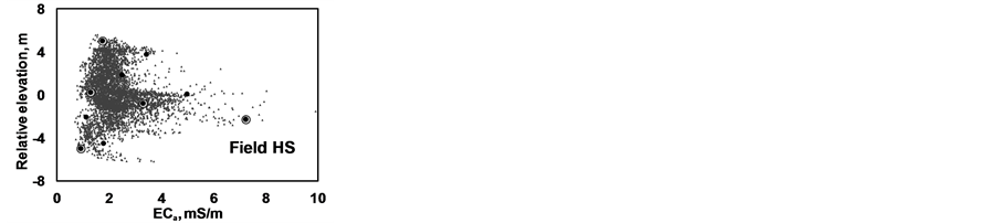
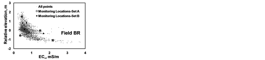
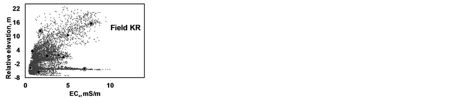
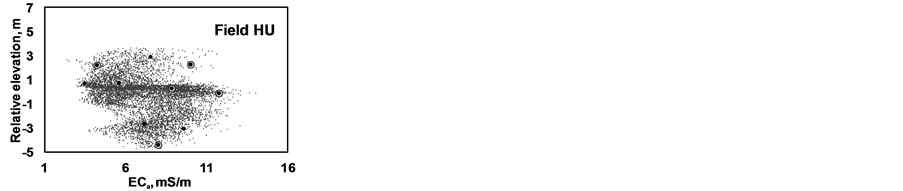
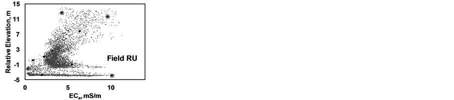
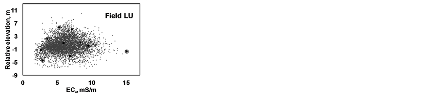
Figure 6. Maps relationship between ECa and field elevation for six fields.
Table 3. Summary of MSE estimates.
Table 4. Percentage of random selections with higher MSE as compared to the optimized selection.
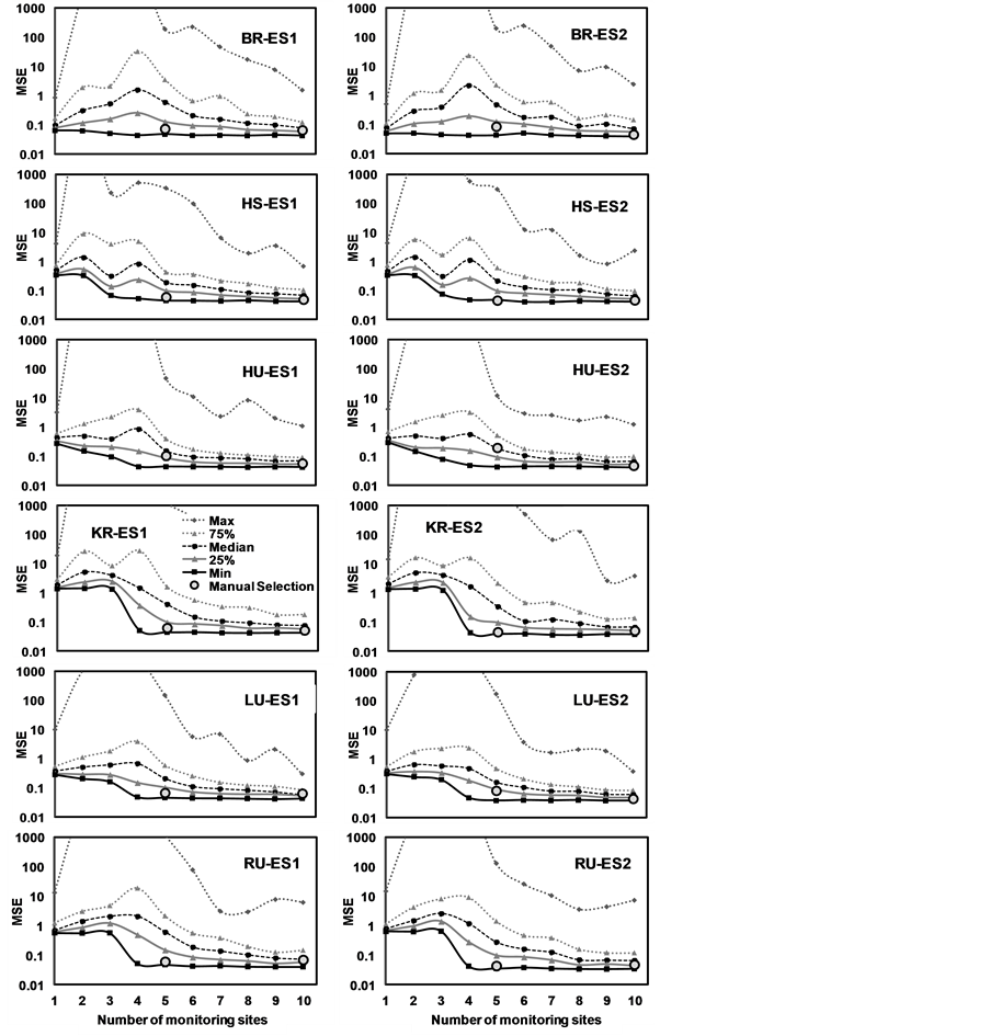
Figure 7. Summary of MSE values for random selection and optimized selection methods for all six fields using simulated surfaces based on error surface (ES 1 and ES 2).
view, this conclusion means that even a small number of monitoring sites can result in a quantification of soil water stress of relatively good quality in every part of the field, as long as these sites are selected carefully and water stress response to soil texture and/or landscape position is well defined. On the contrary, using a small number of monitoring sites to define parameters of a complex regression model greatly increases the chance of errors in estimating these parameters which would lead to lower WSP predictability.
Depending on the cost of added monitoring sites and the profit-reducing effect of WSP prediction errors, the optimum number of these sites will be different. Thus, errors in estimating water stress levels will lead to yield loss due to water stress and/or the extra cost of unnecessary water supply. Based on Equation (5), we anticipate that a single monitoring site placed in the most representative part of the field is a valid starting point. When soil variability, or field topography, presents a case for a substantial differences in expected plant available water storage, two monitoring locations are required. Once both soil ECa and field elevation change substantially and do not correlate, three monitoring locations are needed. Once the interaction between the two high-density data layers is also influential, this supports the addition of a fourth monitoring site. However, due to the fact that the relationship between high-resolution data and WSP (Equation (5)) is not certain, extra monitoring sites could assure a more accurate definition of regression parameters, which should be fewer in number than the number of monitoring locations.
Based on this research, the greater the number of monitoring locations that can be equipped, the lower probability of selecting a set of locations with poor quality of regression parameters prediction will be. Once the number of monitoring locations is large, it is not as critical to seek the most appropriate locations as compared to a low number of such sites. With a relatively small number of temporal soil water monitoring sites (due to economic restrictions), the optimized site selection strategy described above can be used as a starting point when developing practical algorithms for irrigators pursuing the benefits of site-specific water management. However, the actual network design algorithm must involve the node communication capabilities, landscape topography, irrigation system geometry, and other infrastructure-based constraints. Some of these network architecture constraints are discussed in [14] .
4. Conclusion
In this study, apparent soil electrical conductivity and field elevation data layers were mapped using on-the-go soil sensing technology. Both data layers were associated with soil water holding capacity. To assess the effect of monitoring site selection, various model WSP surfaces were obtained by adding up the calculated WSP and an error simulated according to different spatial distribution patterns. The random selection method and the optimized selection method based on specified criteria were applied and compared on the basis of the MSE computed from the predicted versus simulated WSP surfaces. The optimized selection of monitoring sites was helpful in reducing the chance of selecting monitoring sites with a poor capacity to recover the WSP regression model. Our results highlight the importance of covering the entire range of spatial data indicating water storage with a high resolution and spreading the sites across the field to account for any additional factors affecting water storage predictability.
Acknowledgements
This research was supported in part by funds provided through the Nebraska Center for Energy Science Research through the Water, Energy and Agriculture Initiative (WEAI); National Science and Engineering Research of Canada (NSERC) Discovery Grant; Agricultural Research Division of the University of NebraskaLincoln; and Deere and Company.
References
- Viscarra Rossel, R.A., Adamchuk, V.I., Sudduth, K.A., McKenzie, N.J. and Lobsey, C. (2011) Proximal Soil Sensing: An Effective Approach for Soil Measurements in Space and Time, Chapter 5. Advances in Agronomy 113, 237-283. http://dx.doi.org/10.1016/B978-0-12-386473-4.00005-1
- Hedley, C. and Yule, I. (2009) A Method for Spatial Prediction of Daily Soil Water Status for Precise Irrigation Scheduling. Agricultural Water Management, 96, 1737-1745. http://dx.doi.org/10.1016/j.agwat.2009.07.009
- Kim, Y., Evans, R.G. and Iversen, W. M. (2009) Evaluation of Closed-Loop Site-Specific Irrigation with Wireless Sensor Network. Journal of Irrigation and Drainage Engineering, 135, 25-31. http://dx.doi.org/10.1061/(ASCE)0733-9437(2009)135:1(25)
- Omary, M., Camp, C.R. and Sadler, E.J. (1997) Center Pivot Irrigation System Modification to Provide Variable Water Application Depths. Applied Engineering in Agriculture, 13, 235-239. http://dx.doi.org/10.13031/2013.21604
- Miranda, F.R., Yoder, R. and Wilkerson, J.B. (2003) A Site-Specific Irrigation Control System. ASABE, St. Joseph, Paper No. 031129.
- Han, Y.J., Khalilian, A., Owino, T.O., Farahani, H.J. and Moore, S. (2009) Development of Clemson Variable-Rate Lateral Irrigation System. Computers and Electronics in Agriculture, 68, 108-113. http://dx.doi.org/10.1016/j.compag.2009.05.002
- Lesch, S.M. (2005) Sensor-Directed Spatial Response Surface Sampling Designs for Characterizing Spatial Variation in Soil Properties. Computers and Electronics in Agriculture, 46, 153-180. http://dx.doi.org/10.1016/j.compag.2004.11.004
- Minasny, B and McBratney, A.B. (2006) A Conditioned Latin Hypercube Method for Sampling in the Presence of Ancillary Information. Computers and Geosciences, 32, 1378-1388. http://dx.doi.org/10.1016/j.cageo.2005.12.009
- Brus, D.J. and Heuvelink, G.B.M. (2007) Optimization of Sample Patterns for Universal Kriging of Environmental Variables. Geoderma, 138, 86-95. http://dx.doi.org/10.1016/j.geoderma.2006.10.016
- de Gruijter, J.J., McBratney, A.B. and Taylor, J. (2010) Sampling for High-Resolution Soil Mapping. Proximal Soil Sensing. Springer Netherlands, 3-14.
- Adamchuk, V.I., Viscarra Rossel, R.A., Marx, D.B. and Samal, A.K. (2011) Using Targeted Sampling to Process Multivariate Soil Sensing Data. Geoderma, 163, 63-73. http://dx.doi.org/10.1016/j.geoderma.2011.04.004
- Pan, L., Adamchuk, V.I., Martin, D.L., Schroeder, M.A. and Ferguson, R.B. (2013) Analysis of Soil Water Availability by Integrating Spatial and Temporal Sensor-Based Data. Precision Agriculture, 14, 414-433. http://dx.doi.org/10.1007/s11119-013-9305-x
- SAS (2008) Optimality Criteria. SAS/QC User’s Guide, SAS Institute Inc., Cary.
- An, W., Ci, S., Luo, H., Wu, D., Adamchuk, V., Sharif, H., Wang, X. and Tang, H. (2013) Effective Sensor Deployment Based on Field Information Coverage in Precision Agriculture. Wireless Communications and Mobile Computing. http://dx.doi.org/10.1002/wcm.2448
NOTES

*Corresponding author.

1Mention of a trade name, proprietary product, or company name is for presentation clarity and does not imply endorsement by the authors, the University of Nebraska-Lincoln, or McGill University, nor does it imply exclusion of other products that may also be suitable.