Journal of Water Resource and Protection
Vol.4 No.7(2012), Article ID:19774,7 pages DOI:10.4236/jwarp.2012.47050
Inverse Modeling of Groundwater Flow of Delta Wadi El-Arish
1Departement for Geology, TU Bergakademie Freiberg, Freiberg, Germany
2Deltares Built Environment and Geosciences, BU Groundwater & Soil Management, Utrecht, The Netherlands
Email: ramawaad@gmail.com
Received March 20, 2012; revised April 24, 2012; accepted May 27, 2012
Keywords: GMS; PEST; LANDSAT
ABSTRACT
Egypt is mainly covered by desert and only 4% of total lands is arable, mainly the alluvial plain of the Nile and its delta. In order to cope with the increasing population, the government of Egypt has been pressed into the development of Sinai Peninsula. So, it is indispensable to evaluate the potential groundwater resources for the development of the Sinai Peninsula. The key components are a conceptual model and a groundwater model with certain mathematical components. The conceptual model is a system analysis of the hydrogeological understanding of how water flows into, through and out of a groundwater system. Based on available borehole data, the study area is characterized to reach to the most representative conceptual models. Finally, a finite difference groundwater model was applied utilizing the graphic user interface GMS were used. In order to handle problems at regional scale, automated parameter estimation (PEST) was used in GMS. Moreover, recharge was parameterized using zones by defining these zones several factors were considered; for example, surface geology, density of vegetation, general land use, and LANDSAT image. However, Groundwater flow model successfully calibrated. Calibrated groundwater model helped to identify the heterogeneity in the aquifer.
1. Introduction
Egypt is located in north-eastern Africa and includes the Sinai Peninsula (also named Sinai), which is often considered as a part of Asia. Egypt’s natural boundaries consist of more than 2900 kilometers of coastline along the Mediterranean Sea, the Gulf of Suez, the Gulf of Aqaba, and Red Sea. Sinai, the triangular-shaped peninsula of Egypt, is situated between Asia and Africa. The separation of the two continents caused the form and geographical shape of Sinai and the way it looks today. Sinai is approximately 380 km long (north-south) and 210 km wide (west-east). The surface area has an extension of 61,000 km2; the coasts are stretching about 600 km to the west and to the east (Figure 1).
Groundwater extracted from wells supply growing population in coastal areas around the world. By 1992 the population of Egypt was 65 million. The population of Egypt is doubling about every 28 years. Egypt has limited water resources. However, water resource must be managed efficiently and wisely to sustain the needs of growing world population. Sinai suffered from water scarcity. North Sinai especially Delta Wadi El-Arish depends on groundwater as a main resource for drink, domestic and agricultural uses etc. Groundwater is the main supply of the water in Delta Wadi El-Arish, yet water level declining due to increasing extraction rates. Many wells dug by the Egyptian Government and Private Sector (Bedouins).
The total length of the Egyptian Mediterranean Sea coast is about 1200 km. The City of El-Arish is the capital and largest city of North Sinai, lying on the Mediterranean coast of the Sinai Peninsula. El-Arish is by a big Wadi called the Wadi El-Arish. Figure 2 shows ElArish City. Egyptian investors to become the leading seashore resort on the Mediterranean Sea have continually enlarged the city.
2. Conceptual Model
The key components of a groundwater model are a conceptual model and a mathematical model. The conceptual model is a descriptive representation of our hydrogeological understanding of how water flows into, through and out of a groundwater system. Based on available borehole data, the study area is characterized to reach to the most representative conceptual models. Most of the data come from the WRRI & Cairo University report [1,2]. Numerous data to characterize the aquifer have been collected in 1988. From these data, three different
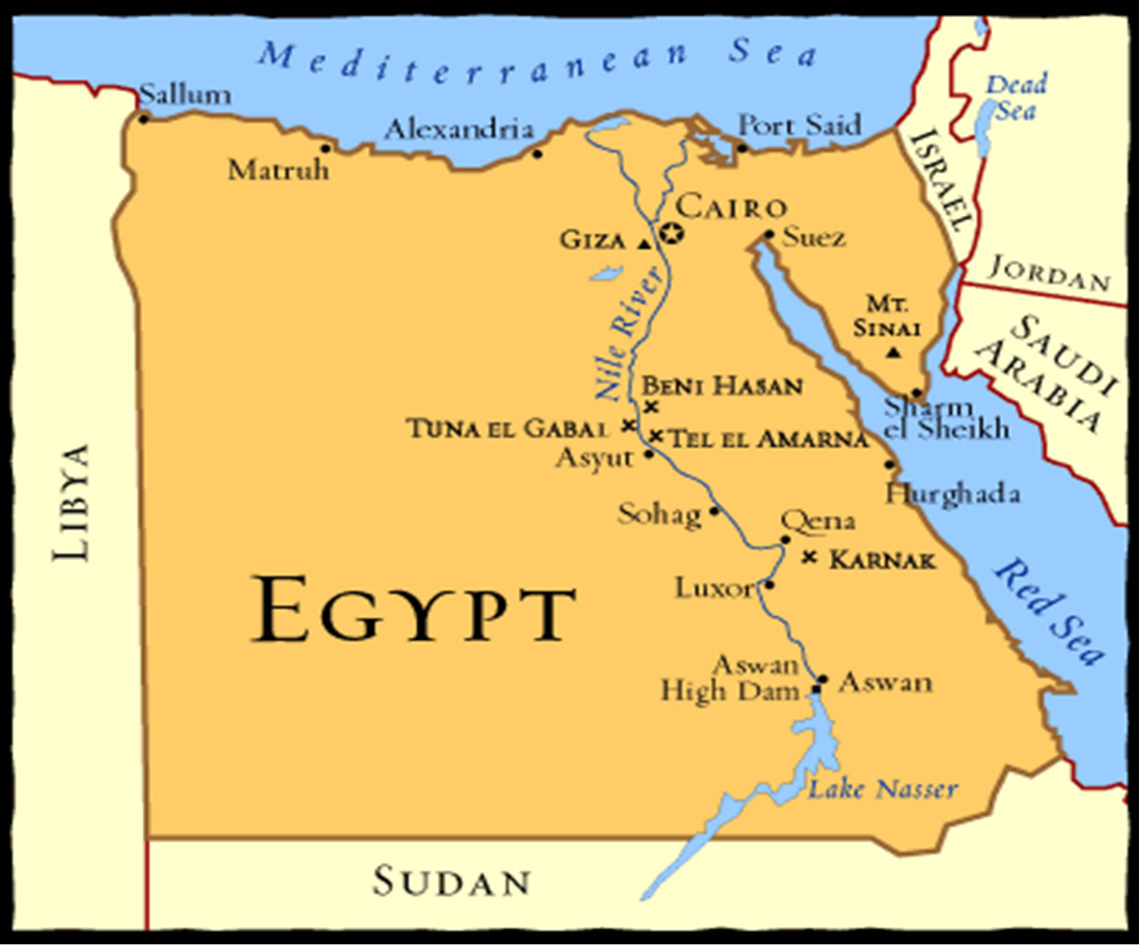
Figure 1. Map of Egypt.

Figure 2. A map of the great El-Arish is located on the Egyptian Mediterranean Sea coast.
formations have been distinguished from a lithological point of view. There are namely:
1) Sand;
2) Gravel and Sand;
3) Calcareous sandstone (Kurkar).
In this paper a monolayer model was adopted. The three layers have been merged to constitute a single equivalent layer with an equivalent permeability, a thickness equal to the sum of the three layer thicknesses.
This approach of an equivalent single monolayer model is consistent with hydraulic head measurements which do not show any significant difference in the two formations. Meanwhile, considering a multilayer model is difficult where there is not enough data to calibrate such model. In this study, calibration is done in a steady state where the evolution of the water levels does not show a significant decrease from 1988 to 1992. So the year 1988 has been chosen to realize a calibration in steady state.
The objectives of this study are calibration groundwater flow in the study area. In addition, minimize the differences between the calculated and measured data using inverse modeling. As well as, come up with solutions to improve water scarcity in the region are provided.
2.1. Forward Modeling
MODFLOW [3] is a public domain, international industry-standard, groundwater modeling software package being used to evaluate the quaternary aquifer of El-Arish area. MODFLOW was applied to construct an equivalent single layer two-dimensional mathematical model of the aquifers under study using all the available hydrogeological, hydrological and pumping and climate data developed from the extensive investigation programs carried out by Water Resources Research Institute (WRRI) & Faculty of Engineering, Cairo University [1,2], and JICA, [4,5]. Figure 3 depicts the computation grid.
2.2. Computational Gird
The Hydrogeological conceptual model is the basis for building the MODFLOW model. Since there are no direct field measurements that support flow in the vertical direction, it is common to adopt a 2-D modeling approach where hydraulic parameters (e.g. hydraulic conductivity) and state variables (e.g. water level) are vertically averaged. Figure 4 shows the 2-D MODFLOW
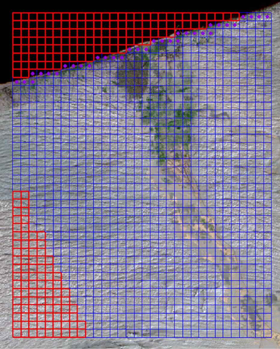
Figure 3. Computational grid overlaid on an infrared false color composition of LANDSAT image acquired on 1987. Inactive cells are shown in red lines.

Figure 4. Cells of abstractions in the study area.
model in a plan view. The model has been constructed with a rectangular grid system of 500 ´ 500 m. It covers an area of 16 km east and 20 km north. The grid size has been selected compromising resolution and computational time. The origin of the grid is (569000.0E, 3428000.0N) in Universal Transverse Mercator (UTM), World Geodetic System (WGS) 1984, zone 36N.
In x-direction a total of 32 cells and in y-direction a total of 40 cells were formed by the grid. The red cells (see Figure 4), however, have later been assigned as being in-active in order to follow the domain borders. The blue cells are active and they form the actual grid system used in the modeling task.
2.3. Boundaries and Boundary Conditions
The Mediterranean Sea borders the model area in the north. So, this boundary is modeled as a constant head boundary. On the east and west side of the model the boundaries are chosen in such a way that they follow the regional direction of the groundwater flow. These two boundaries are modeled as No-flow boundary. In the south, impervious boundary corresponding to the limit of the aquifer extension has been taken into account leading to adopting a No-flow boundary. However, only the inlet of Wadi El-Arish at the south boundary of the study area has been considered as flow boundary whose value is obtained from [6].
3. Steady State Calibration
Generally stated, the inverse problem may be defined as estimating a set of relevant flow parameters given: 1) point measurements of the flow parameters; 2) some hydrological measurements collected during a flow experiment; along with 3) any other (possibly transient) measurements which are sensitive to flow processes, including geophysical measurements. A solution to this inverse problem is the parameter distribution for which the simulated and measured observational data match, and which preserves parameter measurements.
In the present study, we assume that the hydraulic conductivity and recharge are unknown flow parameters. Although recharge and hydraulic conductivity are both spatially variable, we assume that only hydraulic conductivity is a randomly variable field. To parameterize such spatially distributed random variable, the Pilot point method is used. The recharge is also assumed spatially variable, but we adopt zonation as a parameterization technique to convert its spatial variability to zones of uniform values.
The success of any inversion depends on the careful choice and implementation of optimization algorithms. Parameter inversion methods are most commonly performed using gradient based methods (e.g., LevenbergMarquardt technique). In GMS (which is an acronym for Groundwater Model System) (the MODFLOW’s preand post-processor used in this study) several alternatives are available to solve the inverse problem. Here, PEST (which is an acronym for Parameter ESTimation) accomplished this task [7]. PEST is a model-independent parameter optimizer. While PEST has some similarities to existing nonlinear parameter estimation software, it has been designed to allow to be interfaced with any model without the necessity of having to make any changes to that model. Doherty [8] suggested use of regularized inversion techniques with practical tools like PEST. PEST is widely use of nonlinear parameter estimation and optimization modeling. More information regarding PEST can be found in [8,9].
3.1. Hydraulic Conductivity
In this study we use water level measurements collected in 1988 to calibrate a steady state model of the study area. As explained by Seguin and Bakr [6] the evolution of the water levels does not show a significant decrease from 1988 to 1992. Water level measurements collected in 1988 counted to 40 data points and are obtained from WRRI & Cairo University report [1]. These water levels range from –3 m (area of pumping) to 2.6 m near the south boundary. Most of the values are below the sea level. When several points were located in a same cell of the model grid, an average value has been considered. Pumping tests data and their interpretation are also available in several reports (e.g., JICA, [4] ). In this light, hydraulic conductivity values vary between 20 and 260 m/d. According to these data, an intermediate value of hydraulic conductivity of 43 m/d has been chosen to assign to the hydraulic conductivity at a set of chosen pilot points.
In 1988 abstraction was approximately 52,000 m3/d where 25,500 m3/d was for domestic use while the rest (26,500) was for irrigation. For the simplest purpose, the model adopt 50% return coefficient for irrigation water at the cells of pumping. Although return water from domestic is also expected, it is necessary not occurring at the locations of pumping wells. Figure 4 shows cells of abstraction in ine modeling grid; note that, those cells at the south east are recharging wells simulating recharge from the inlet of the Wadi to the study area.
3.2. Recharge
Spatially distributed recharge also exists in the study area. There are several sources of such recharge including infiltration from rainfall, return water from the imported Nile water to the area, and recharge due to domestic water use. In 1988, the imported water from the Nile was about 10,450 m3/d. Meanwhile, average rainfall in the study area is estimated as 105 mm/yr for the period between 1936 and 1967; see Cairo University Report [1]. Also, vegetation and their distribution may have impacted on the amount of distributed recharge through evaporation and other processes that may take place in the vadose zone even though that irrigation return coefficient implemented in the point sink items in the model.
3.3. Calibration Parameters
Simultaneously recharge and hydraulic conductivity were calibrated. The recharge is parameterized using zones. In defining these zones several factors were considered; for example, surface geology, density of vegetation and general land use. Here, LANDSAT image acquired in 1986 was used to identify these zones. The image is composed using bands 7, 4 and 2 present a shortwave false color composition where vegetation appears in green and urban areas appear in dark lavender. Figure 5 shows different zones of recharge where their values are to be estimated in the calibration. Values of hydraulic conductivity at those points are to be estimated in the calibration of the model.
3.4. Calibration Results
As stated before, the calibration target of this study was to calibrate the spatially variable hydraulic conductivity and recharge. Calibration was done iteratively which lasted for 16 iterations and gave 8.55 sum squared weighted

Figure 5. Recharge zones.
residuals (all dependent variables). Figure 6 shows computed versus observed heads. The figure shows very good results for all of the observation points.
Figure 7 shows calibrated parameters where it shows recharge and log-transformed hydraulic conductivity Figure 8. The figure shows that recharge varies between 1.62 × 10⁻⁵ m/d which exists in areas of recharge due to infiltration solely from rainfall and 3.5 × 10⁻³ m/d which comprises combination effects of rainfall, irrigation and other possible sources that are not accounted for directly in this study. The estimated recharge is about 0.0002 m/d. This corresponds to about 10% of the total domestic abstraction.
Also, Figure 8 shows the log-transformed hydraulic conductivity (ln(K)). The figure shows that the calibrated (ln(K)) ranges between –0.15 and 5.05 (this corresponds to 0.86 and 156 m/d). It shows that the middle part of the study area has the minimum to average hydraulic conductivity while higher values exist in west-north and middle-east of the study area.
Finally, Figure 9 shows calibrated piezometeric heads for 1988. The figure shows that the aquifer is subject to aggressive pumping where many locations of negative water levels do exist.
Table 1 shows volumetric budget for the entire model at 1988 assuming a steady state solution. The table shows that the long-term average for recharge is 34228.8 m/d. It also shows that there are local salt water intrusions that amount only 9381.6 m/d.

Figure 6. Calibration results: computed versus observed heads.
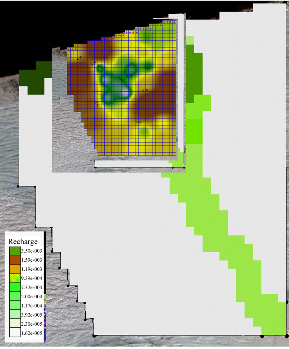
Figure 7. Calibration results: recharge.
4. Transit Simulation
In this section we examine transient flow in the period between 1988 and 2006. Based on available pumping rates and locations of wells in 1988 and 2006, linearly interpolate the rates for a yearly stress period. This gives 18 stress periods. This linear interpolation assumption is consistent with available data for irrigation and domestic wells between 1988 and 2006 where they show a trend of linear relationships. Amount of abstraction introduced in
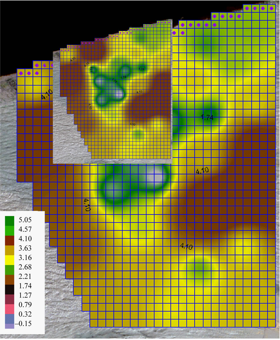
Figure 8. Log-transformed hydraulic conductivity.
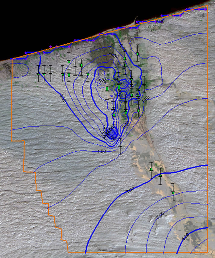
Figure 9. Calibrated water level for 1988. Green bars indicate the difference between calibrated and measured water levels.
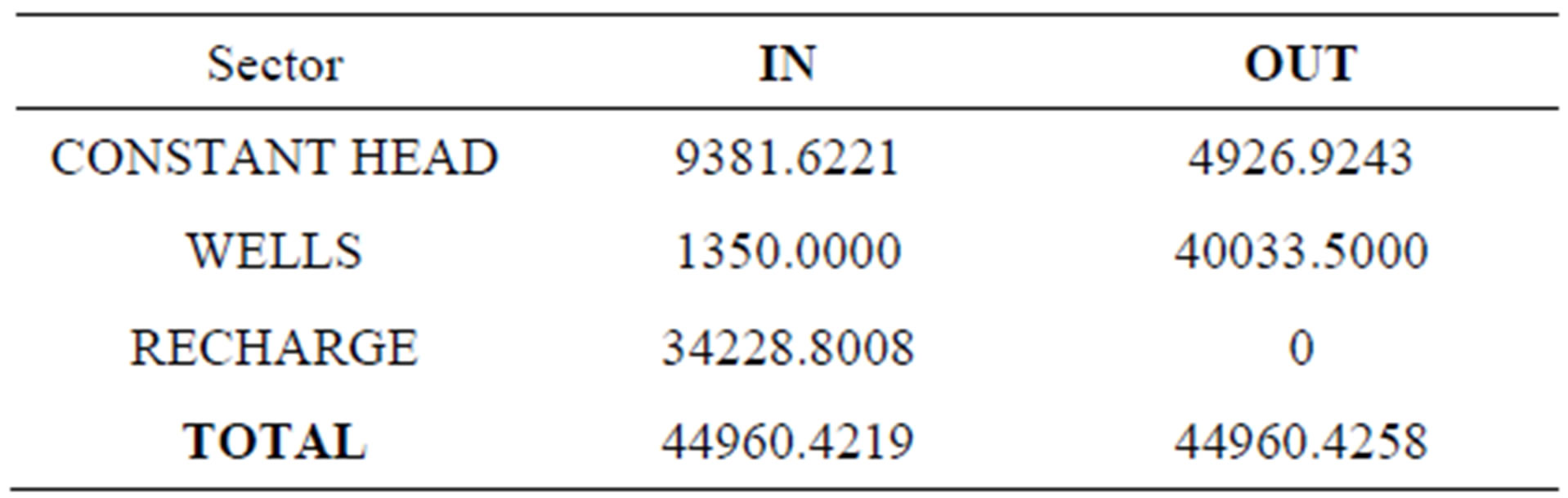
Table 1. Volumetric budget for the entire model at 1988 assuming steady state.
the model of this study for the year 2006 in this study is 52555 m3/d. Figure 11 and Figure 10, Piezometric level time series for cells within the urban area of El-Arish city The model assumed that calibrated recharge, presented in the previous section, is constant over the simulation period between 1988 and 2006. However, in this study the recharge was changed in urban areas to zero as the sewerage system in El-Arish city has started operating in 2002. Figures 10-11 show the time series of piezometric water level of two cells in the study area. The figures show a cell in the urban area of El-Arish city and a cell in the agriculture area close to the airport, almost in the middle of the study area. Both plots show a drop in water levels between 0.6 m and 0.75 m. The graph of the urban area also shows a sudden drop in 2002 due to the return of the domestic water use which led to the stopping recharging.
Such drops in the water level indicate possible sea water intrusion, which is also supported by the volumetric water balance given in Table 2. Finally, this also can
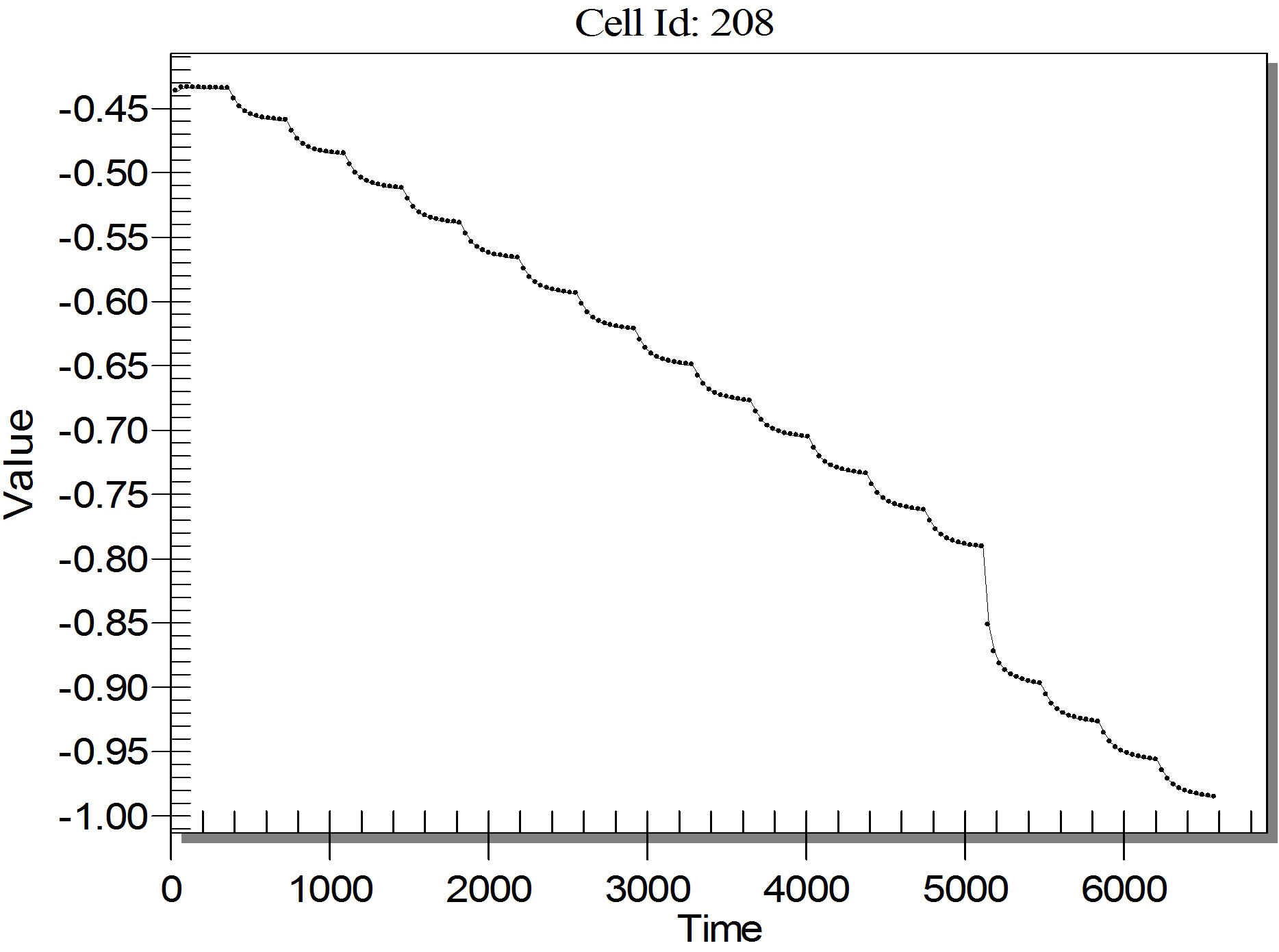
Figure 10. Piezometric level time series for a cell within the urban area of El-Arish city.

Figure 11. Piezometric level time series is for a cell almost middle of the study area.

Table 2. Volumetric budget for entire model at end of time step 10 in stress period 18.
be anticipated from the simulated piezometeric levels for 2006 shown in Figure 12.
Due to the nature of the aquifer constituents in El- Arish area which contains sand, gravel and silt that gives a chance to be polluted by different sources where the infiltration rate increases and affect to the groundwater quality.
From two years ago, there is no complete drainage system at El-Arish city. The amount of drainage water is estimated by the amount of about 45.000 m3, which acts as a natural obstruction against the seawater intrusion especially the wells near the coast.
Therefore, the general strategy to protect the health and environment should be including many of infrastructures which decrease or prevent the pollution sources.
5. Conclusions and Recommendation
From the previous study, it clears that there is a deterioration in the groundwater levels decline in El-Arish area, which indicates that the abstraction amounts are exceeding the natural recharge which depending mainly on the annual amount of rainfall. Therefore, the water balance is in critical situation which needs an improved management to exploit the water resources. Hence, the laws and restrictions should be present to prevent drilling extra wells. The government supplies El-Arish area by 25.000 m3/day uses in the domestic uses to meet the expected increase in population. The abstraction rate exceeding the recharge rates which cause an increasing in water salinity.

Figure 12. Simulated piezometeric levels in 2006.
The main conclusions are as follows:
• The model matches the available data quite well.
• Inverse modeling with a PEST provides to be a unique tool to calibrate groundwater modeling.
• The density driven model should be carried out in the future to get a better understanding about the saltwater intrusion.
The main recommendations are as follows:
• The option to desalinate water from seawater and the existing wells should be considered as an economic solution in the future. It is recommended due to its medium cost which between 5 to 10 Egyptian pounds.
• Solar desalination is unique solution spatially in this area which desalinates water using solar energy.
• The transported Nile water should be increased to cover the water demands of population growth.
• A network should be constructed to connect all the water wells working with electricity to work automatically.
Increasing of environmental awareness to the public is needed to keep the water clean and avoid pollution of groundwater aquifer.
REFERENCES
- Faculty of Engineering, Cairo University, “Groundwater Management Study in El-Arish Rafaa Plain Area,” Phase 1, Main Report, Vol. 1, Water Resources Research Institute, Ministry of Public Works and Water Resources, 1989.
- Faculty of Engineering, Cairo University, “Geological Sounding Survey in El-Arish, Sheikh Zuwyied, Rafah Area,” Main Report, Vol. 1, Water Resources Research Institute, Ministry of Public Works and Water Resources, 1989.
- A. W. Harbaugh, E. R. Banta, M. C. Hill and M. G. McDonald, “MODFLOW-2000, the US Geological Survey Modular Ground-Water Model—User Guide to Modularization Concepts and the Ground-Water Flow Process,” US Geological Survey Open-File Report 00-92, 2000.
- JICA, North Sinai, “Groundwater Resources Study in the Arab Republic of Egypt,” Final Report, 1992,
- A. Shata, “Groundwater and Geomorphology of the Northen Sector of Wadi El Arish Basin,” Bulletin Society Geograph Egypt, Vol. 32, 1959.
- J. J. Seguin and M. Bakr, “Sinai Water Resources Study, Modelling of Three Aquifers: El Arish, Rafah, and El Qaa,” WRRI, NWRC, Egypt, 1992.
- J. Doherty, “PEST: Model-Independent Parameter Estimation,” Watermark Computing, 1994.
- J. Doherty, “Manual and Addendum for PEST: Model Independent Parameter Estimation,” Watermark Numerical Computing, Brisbane, 2008.
- J. Doherty, “Ground Water Model Calibration Using Pilot Points and Regularization,” Ground Water, Vol. 41, No. 2, 2003, pp. 170-177. doi:10.1111/j.1745-6584.2003.tb02580.x