Journal of Water Resource and Protection
Vol. 3 No. 11 (2011) , Article ID: 8680 , 7 pages DOI:10.4236/jwarp.2011.311090
Calibration of HEC-RAS Model on Prediction of Flood for Lower Tapi River, India
1Department of Civil Engineering, S. V. National Institute of Technology, Surat, India
2S. V. National Institute of Technology, Surat, India
E-mail: {pvtimbadiya, plpatel}@ced.svnit.ac.in, pdporey@svnit.ac.in
Received August 28, 2011; revised September 30, 2011; accepted October 27, 2011
Keywords: Hydrodynamic model, calibration, simulation, flood and stage hydrograph, Validation, HEC-RAS
ABSTRACT
Channel roughness is a sensitive parameter in development of hydraulic model for flood forecasting and flood inundation mapping. The requirement of multiple channel roughness coefficient Mannnig’s ‘n’ values along the river has been spelled out through simulation of floods, using HEC-RAS, for years 1998 and 2003, supported with the photographs of river reaches collected during the field visit of the lower Tapi River. The calibrated model, in terms of channel roughness, has been used to simulate the flood for year 2006 in the river. The performance of the calibrated HEC-RAS based model has been accessed by capturing the flood peaks of observed and simulated floods; and computation of root mean squared error (RMSE) for the intermediated gauging stations on the lower Tapi River.
1. Introduction
With rapid advancement in computer technology and research in numerical techniques, various 1-D hydrodynamic models, based on hydraulic routing, have been developed in the past for flood forecasting and inundation mapping. The discharge and river stage were chosen as the variables in practical application of flood warning [1]. The discharge, river stage and other hydraulic properties are interrelated and depend upon the characteristics of channel roughness. Estimation of channel roughness parameter is of key importance in the study of openchannel flow particularly in hydraulic modeling. Channel roughness is a highly variable parameter which depends upon number of factors like surface roughness, vegetation, channel irregularities, channel alignment etc. [2]. Several researchers including Patro et al. [3], Usul and Turan [4], Vijay et al. [5] and Wasantha Lal A. M. [6] has calibrated channel roughness for different rivers for the development of hydraulic model. Datta et al. [2] estimated single channel roughness value for open channel flow using optimization method, taking the boundary condition as constraints. The channel roughness is not a constant parameter and it varies along the river depending upon variation in channel characteristic along the flow. The field visit from Ukai to the Surat city, see Figures 1, 2, 3 and 4 was undertaken and the variation in channel roughness along the river was observed in the present study. This clearly demonstrates the variation in channel roughness along the natural river. The Surat city, being coastal city, had been seen susceptible to major floods and undergone with huge damage in the past. For
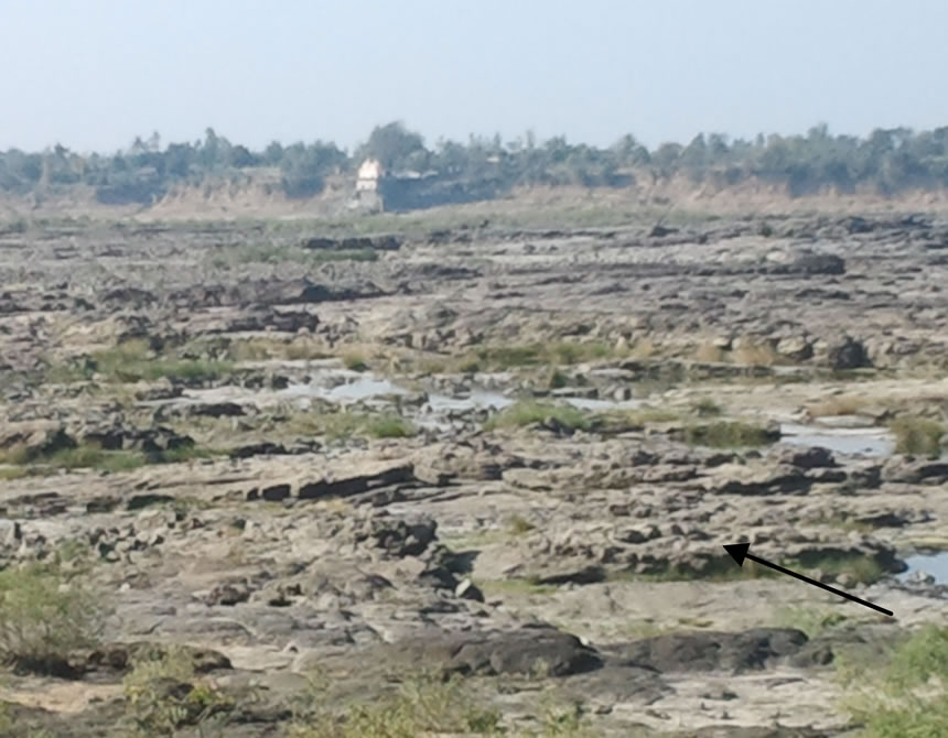
Figure 1. Channel characteristic in upper part of the lower Tapi River (Location: Kakrapar weir).
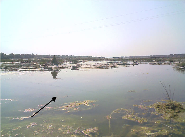
Figure 2. Channel characteristic in middle part of the lower Tapi River (Loaction: Mandavi bridge).
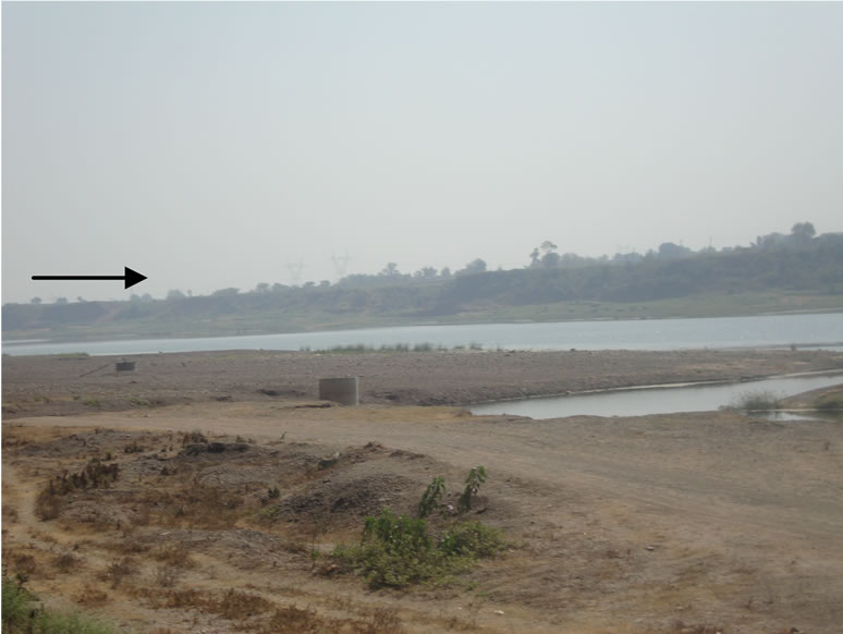
Figure 3. Channel characteristic in middle part of the lower Tapi River (Location: Ghala).
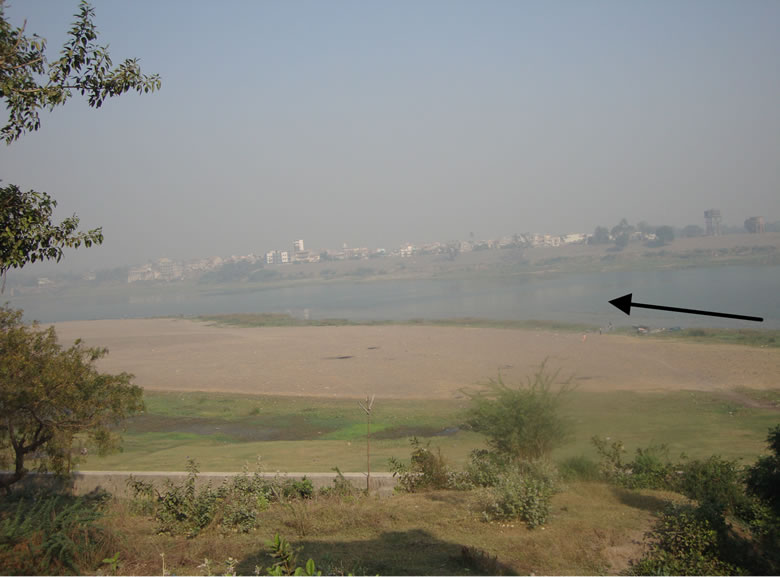
Figure 4. Channel characteristic in lower part of the lower Tapi River (Loaction: Kathor bridge).
example, the flood for year 2006 alone had caused a direct damage to the tune of US $ 4200 million to the nation and whole city remained submerged for more than two days [7]. Thus, at present, there is an urgent requirement of a hydrodynamic model which should be able to predict the flood levels in the lower part of the Tapi River for flood forecasting and protection measures in and around the Surat city. Accordingly, channel roughness for the lower Tapi River (Ukai dam to Hope Bridge) has been calibrated using stream flow data of the past floods, i.e. flood of year 1998 and 2003. The calibrated model has been used to simulate the flood for year 2006 for the same reach.
2. Model Description
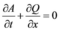
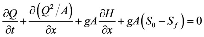
In the present study, unsteady, gradually varied flow simulation model i.e. HEC-RAS, which is dependent on finite difference solutions of the Saint-Venant equations (Equations (1), (2)), has been used to simulate the flood in the lower Tapi River.
 (1)
(1)
 (2)
(2)
here A = cross-sectional area normal to the flow; Q = discharge; g = acceleration due to gravity; H = elevation of the water surface above a specified datum, also called stage; So = bed slope; Sf = energy slope; t = temporal coordinate and x = longitudinal coordinate. Equations (1) and (2) are solved using the well known four-point implicit box finite difference scheme [8]. This numerical scheme has been shown to be completely non-dissipative but marginally stable when run in a semi-implicit form, which corresponds to weighting factor (q) of 0.6 for the unsteady flow simulation. In HEC-RAS, a default θ is 1, however, it allows the users to specify any value between 0.6 to 1. The box finite difference scheme is limited to its ability to handle transitions between subcritical and supercritical flow, since a different solution algorithm is required for different flow conditions. The said limitation is overcome in HEC-RAS by employing a mixed-flow routine to patch solution in sub reaches [8].
3. Study Reach
The Tapi river, the second largest west flowing river in India, originates from Multai (Betul district) in Madhya Pradesh (M.P.) at an elevation of 752 m having length of 724 km and falls in to the Arabian Sea at little beyond the Surat city. The total drainage area of Tapi is 65,145 km2 out of which 9804 km2 lies in Madhya Pradesh, 51,504 km2 lies in Maharastra and 3837 km2 lies in Gujarat. The basin has elongated shape with maximum length of 687 km from east to west and maximum width of 210 km from north to south, see Figure 5. The Tapi basin is divided in three sub-basins namely, upper Tapi basin (up to Hathnur), middle Tapi basin (Hathnur to Gighade) and lower Tapi basin (Gighade to the sea). The Surat city is located at the delta region of the Tapi river [9].
Geometric and Hydrologic Data
The Channel geometry, boundary conditions and channel resistance are required for conducting flow simulation through HEC-RAS. The Surat Municipal Corporation (SMC) has provided the geometric data of the reach for present study as contour map in Auto CAD (.dwg file) format. The cross-section data at different locations were extracted from aforesaid map for the river under consideration. The study reach is about 120 km long and has very mild slope. The effect of meandering has been neglected as there is no reasonable curvature seen in study reach by providing expansion and contraction coefficient as 0.3 and 0.1 respectively. Total 139 cross-sections at various important locations on the river have been used. The Flood hydrograph at Ukai dam and stage hydrograph at Hope bridge (Surat city) have been considered as upstream and downstream boundary conditions respectively. The detailed configuration of Singanpur weir and Kakrapar weir were respectively collected from SMC and Surat Irrigation Circle (SIC), Govt. of Gujarat, India in the hard map format. The discharge coefficient of Kakrapar weir (crest width = 2.4 m and ogee shape) and Singanpur weir (crest width = 10 m and broad crested shape) were computed to be 1.88 and 1.67 respectively [10].
The Central Water Commission (CWC) provided stage data for both Ghala and Hope bridge station for preset simulation. However, SIC has provided the hourly outflow and hourly stage data for Ukai dam and stage data for Kakrapar weir for present investigation. State Water Data Centre (SWDC) has provided the hourly water level for Mandavi station. Also, field study was undertaken to observe the bed condition of the lower Tapi River from Ukai dam to the Surat city. The typical photographs taken during the visit of lower stretch of the Tapi River are shown in Figures 1, 2, 3 and 4.
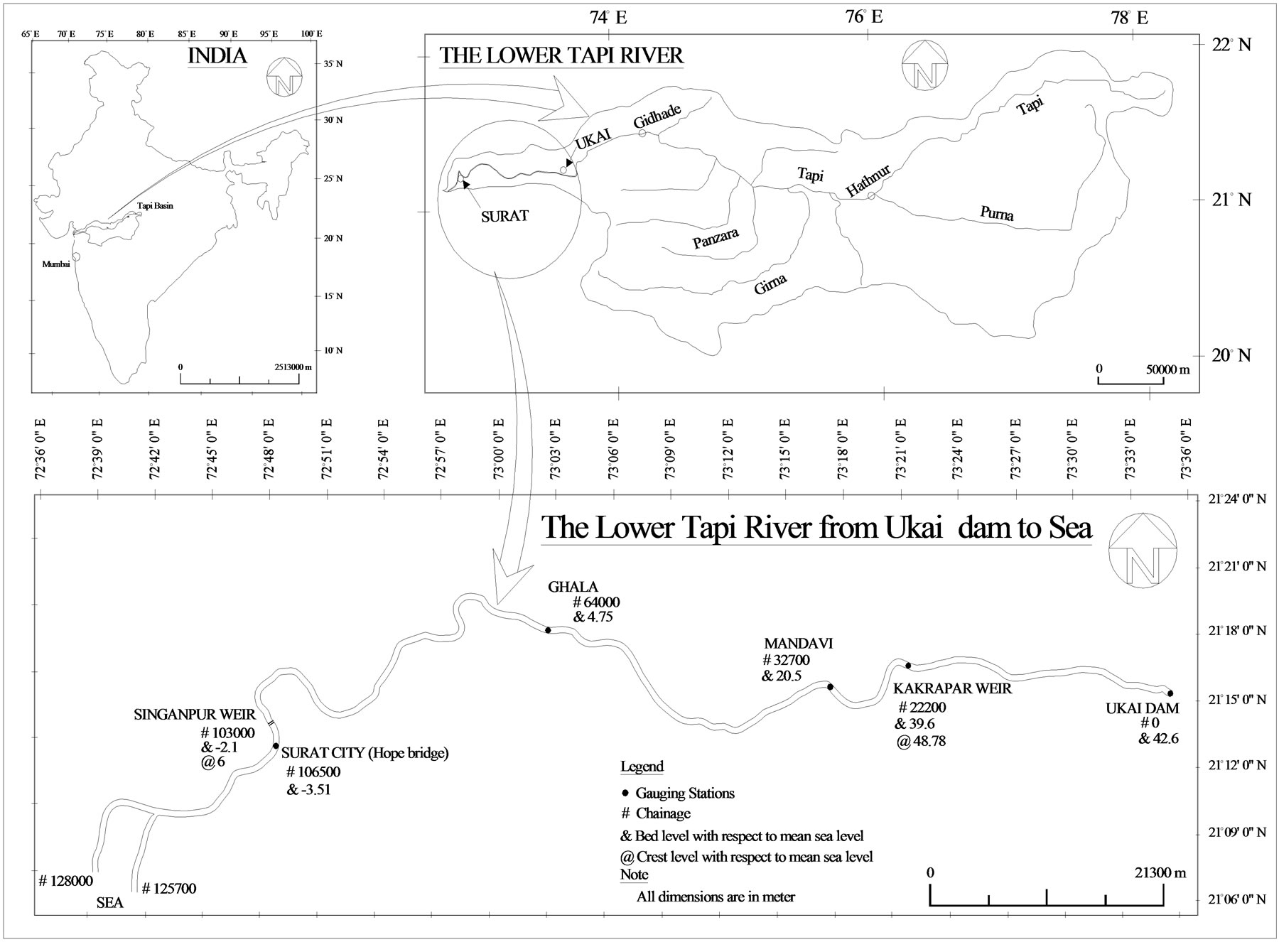
Figure 5. Index map of the Tapi basin and the Tapi River.
4. Calibration of HEC-RAS for Manning’s Roughness Coefficient ‘n’
The data pertaining to the floods for years 1998 and 2003 have been used for calibration of Manning’s roughness coefficient, ‘n’, and using the same in simulation of future floods in the lower Tapi River from Ukai dam to Hope bridge. The photographs shown in Figures 1 to 4 clearly demonstrate that taking single ‘n’ value for simulation of flood in the whole reach would not be appropriate. Firstly, effort has been made to calibrate Manning’s roughness coefficient for single value using aforesaid data and, subsequently, different values have been used to justify their adequacy for simulation of flood in the study reach. Various single values used in calibration for whole reach for floods of years 1998 and 2003 are shown in Table 1. The table, also, shows the flow duration and data for various gauging stations for calibration and validation in foregoing investigation.
5. Simulation of Stages and Flow for Different Value of Manning’s ‘n’
The HEC-RAS model of the lower Tapi River (Ukai dam to Hope bridge) has been used to simulate the stages for different single roughness coefficients (Manning’s ‘n’)
for floods of year 1998 and 2003. Different values of Manning’s ‘n’ (single value for whole reach) have been used, as shown in Table 1, to arrive some optimal value for aforementioned model. The simulated stage hydrographs were compared with observed stage hydrograph at Kakrapar weir, Mandavi and Ghala stations. Simulation periods used for floods of different years are also enumerated in Table 1. Root mean squared error (RMSE) has been used for comparison of simulated stage with observed stage for various Manning’s ‘n’ listed in Table 1.
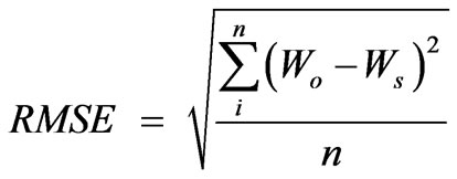
RMSE can be defined as,
 (3)
(3)
where Wo = observed water level in meter (above Mean Sea Level), Ws = simulated water level in meter and n = total no. of reference data points. Comparison of observed and simulated stage hydrographs using aforementioned performance index for flood of years 1998 and 2003 are shown in Tables 2 and 3 respectively. From Table 2, it is apparent that there is no single value of Manning’s ‘n’ can be chosen which may give best performance for all the gauging stations. For example, n = 0.035 better performance is achieved for Kakrapar weir while n = 0.020 gives better performance for Mandavi
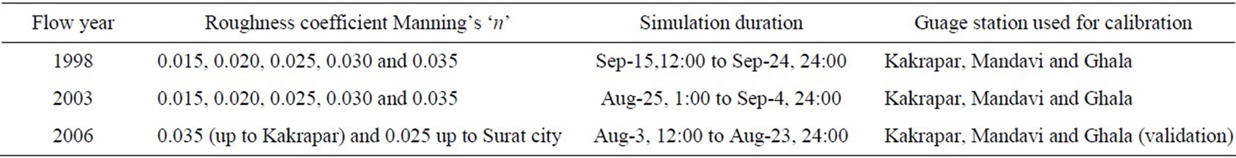
Table 1. Flow duration, Manning’s ‘n’ and gauge station used for calibration and validation.
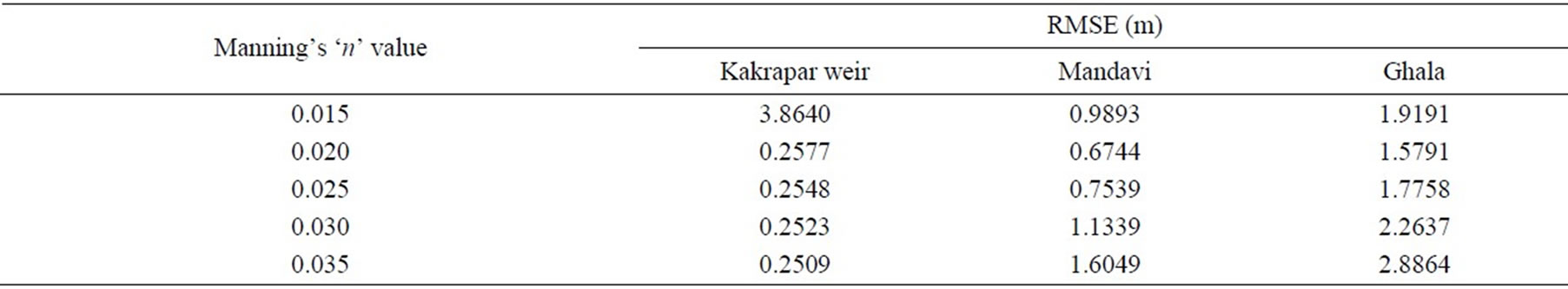
Table 2. Comparison of stage hydrograph for different Manning’s ‘n’ for year 1998.
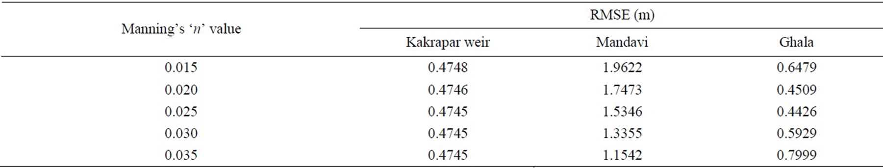
Table 3. Comparison of stage hydrograph for different Manning’s ‘n’ for year 2003.
and Ghala stations. Similarly, for flood of year 2003 (Table 3), it can be seen that model gives better results for Kakrapar for n = 0.035 while the same is true for Mandavi and Ghala stations for n = 0.025. Thus, keeping in view, the topographic survey of river bed features and aforesaid analysis, it can be concluded that single ‘n’ value for the whole reach in foregoing simulation would not be appropriate. Thus, there is no single value can be chosen for simulating the flood for whole reach.
Accordingly, two different values of ‘n’ were considered in calibration of HEC-RAS model, i.e., n = 0.035 up to Kakrapar weir and n = 0.015/0.020/0.025/0.030 downstream of Kakrapar weir. The performance of the model for aforesaid conditions is shown in Tables 4 and 5 respectively, for flood of years 1998 and 2003.
Also, the optimal values of ‘n’ (downstream of Kakrpar weir) which give best results are plotted in Figure 6 for all the gauging stations along the river. From Tables 4, 5 and Figure 6, it can be inferred that the model performs reasonably well for n = 0.035 up to Kakrapar weir while n = 0.025 for downstream of Kakrapar weir. Also, comparison of results in Tables 2-4 and 3-5, clearly indicate that RMSE value are better in flood simulation with two ‘n’ values as compared to single value being taken for the whole reach.
6. Performance of Calibrated Model in Simulation of Flood for Year 2006
The calibrated HEC-RAS based model has been used to simulate the flood for year 2006. The comparison of observed and simulated stages at Kakrapar weir, Mandavi and Ghala gauging stations are shown in Figures 7, 8 and 9 respectively while comparison of observed flood hydrograph with simulated flood hydrograph at Kakrapar weir is also shown in Figure 10.
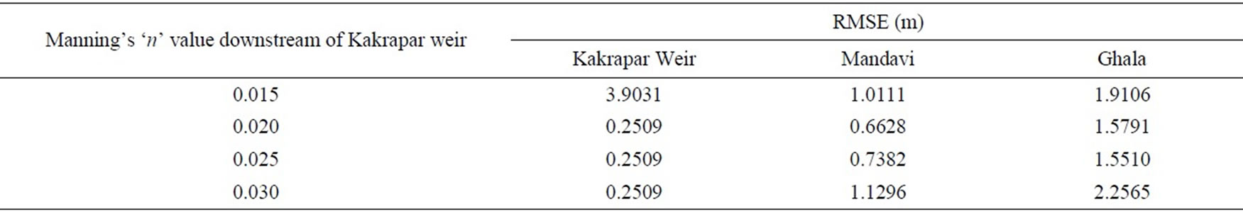
Table 4. Comparison of stage hydrograph for different Manning’s ‘n’ (n = 0.035 up to Kakrapar weir) for year 1998.
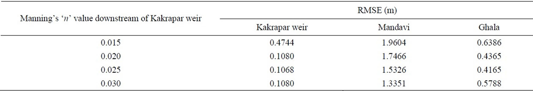
Table 5. Comparison of stage hydrograph for different Manning’s ‘n’ (n = 0.035 up to Kakrapar weir) for year 2003.
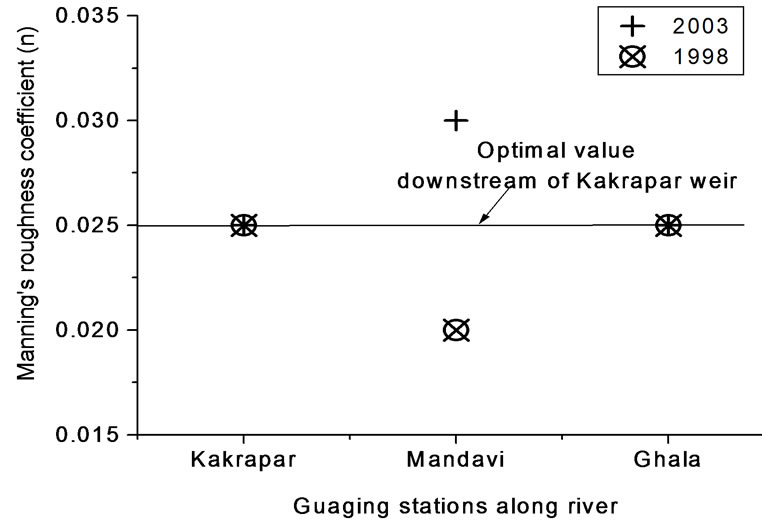
Figure 6. Optimal value of Manning’s roughness ‘n’ for different gauging stations on the lower Tapi River (n = 0.035 up to kakrapar weir).
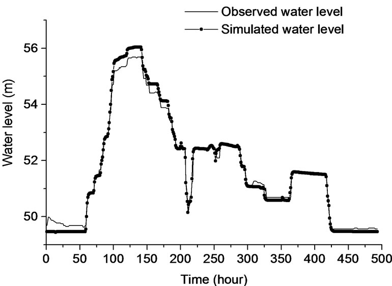
Figure 7. Observed and simulated stage hydrograph at Kakrapar weir for year 2006.
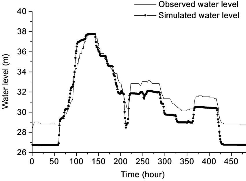
Figure 8. Observed and simulated stage hydrograph at Mandavi for year 2006.
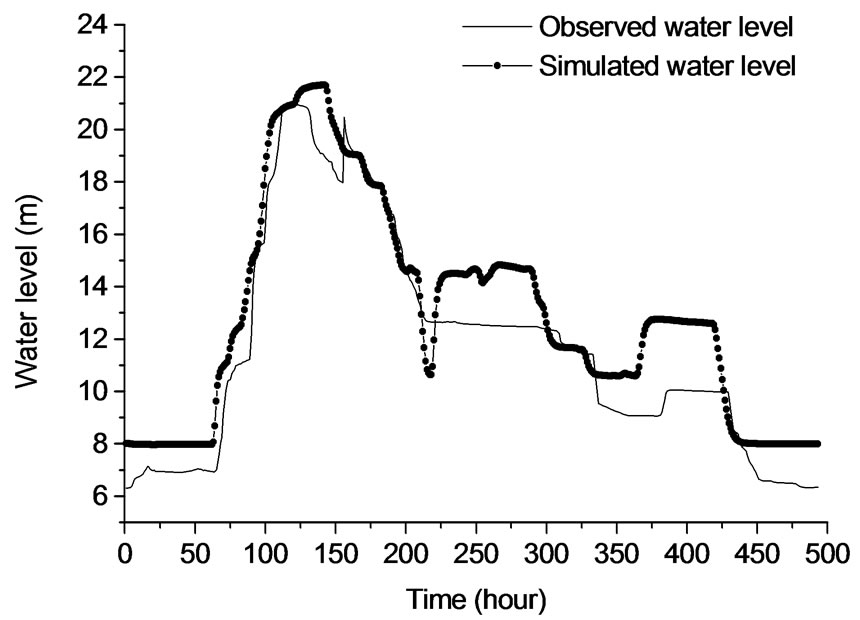
Figure 9. Observed and simulated stage hydrograph at Ghala for year 2006.
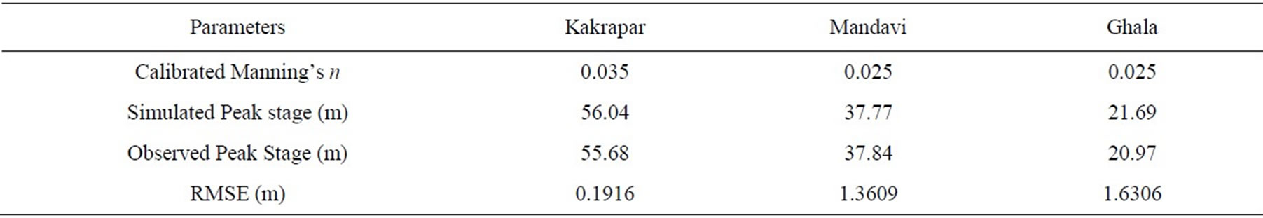
Table 6. Performance of calibrated model in flood year 2006 prediction.
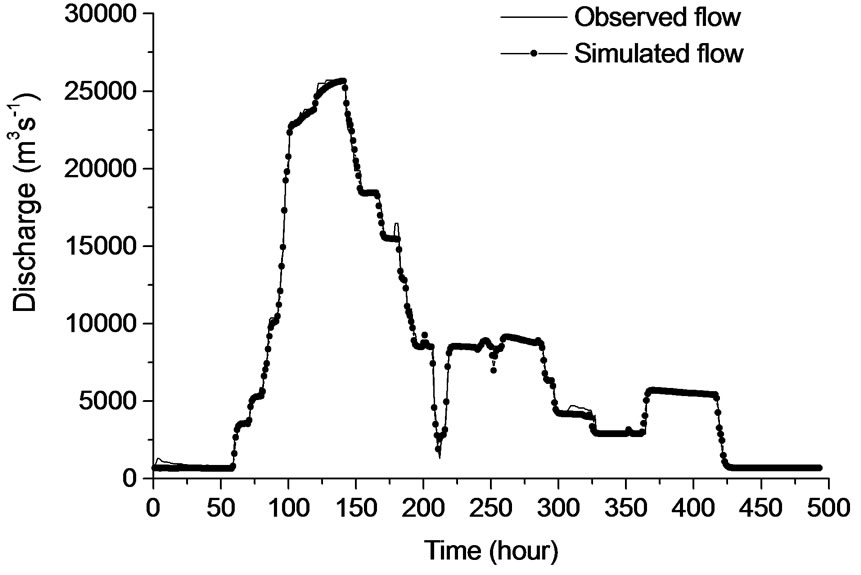
Figure 10. Observed and simulated flow hydrograph at Kakrapar weir for year 2006.
Also, the RMSE has been computed to access the performance of model in stage prediction for all the three gauging stations, viz., Kakrapar, Ghala and Mandavi stations, see Table 6. The table also shows the performance of the model in simulating the peak stage for all the three stations.
The results of simulated stage hydrographs, Figures 7-9, and Table 6 are in good agreement with observed stage hydrographs for flood of year 2006. The performance of calibrated model is better at Kakrapar weir than those with Mandavi and Ghala stations. This may be ascribed to the fact that flood of year 2006 was within the banks of river in upper region (Kakrapar weir) and spread through either bank in lower region (Mandavi and Ghala) where in the flow became two dimensional in nature. Also, the simulated and observed peak stages are in order as enumerated above. The simulated flood hydrograph is in close agreement with observed hydrograph at Kakrapar weir, see Figure 10.
7. Conclusions
On the basis of assessment of topographic features of the lower Tapi River (Ukai dam to Hope Bridge) and simulation of past floods, following findings can be summarized in brief:
1) Topographic assessment of river bed features and simulation of past floods of year 1998 and 2003 for single value of Manning’s roughness coefficient, it became evident that different Manning’s roughness coefficients are required for upper and lower reaches of the lower Tapi River for simulation of flood.
2) Further, simulation of aforesaid flood for multiple values of Manning’s roughness coefficient along the river reach has revealed that a value n = 0.035 up to Kakrapar weir and n = 0.025 downstream of Kakrapar weir would be suitable for simulation of future flood in the lower Tapi River.
3) The performance of calibrated model has been verified for flood of year 2006. Close agreement have been arrived between simulated and observed stages for Kakrapar gauging station. However, the performance is reasonably good for Mandavi and Ghala gauging stations.
4) Furthermore, two dimensional hydrodynamic model of the lower Tapi River including its flood plain area is required to improve the results further.
8. Acknowledgements
Authors acknowledge the All India Council for Technical Education, New Delhi for financial support to carry out the said work under the Nationally Coordinated Project on “Development of Water Resources and Flood Management Centre at SVNIT-Surat”. Authors are also grateful to Central Water Commission (Govt. of India), Surat Irrigation Circle (Govt. of Gujarat, India), State Water Data Centre (Govt. of Gujarat, India) and Surat Municipal Corporation for providing data to carry out the present investigation.
REFERENCES
- W.-M. Bao, X.-Q. Zhang and S.-M. Qu, “Dynamic Correction of Roughness in the Hydrodynamic Model,” Journal of Hydrodynamics, Vol. 21, No. 2, 2009, pp. 255-263. doi:10.1016/S1001-6058(08)60143-2
- R. Ramesh, B. Datta, M. Bhallamudi and A. Narayana, “Optimal Estimation of Roughness in Open-Channel Flows,” Journal of Hydraulic Engineering, Vol. 126, No. 4, 1997, pp. 299-303. doi:10.1061/(ASCE)0733-9429(2000)126:4(299)
- S. Patro, C. Chatterjee, S. Mohanty, R. Singh and N. S. Raghuwanshi, “Flood Inundation Modeling Using Mike Flood and Remote Sensing Data,” Journal of the Indian Society of Remote Sensing, Vol. 37, No. 1, 2009, pp. 107- 118. doi:10.1007/s12524-009-0002-1
- N. Usul and T. Burak, “Flood Forecasting and Analysis within the Ulus Basin, Turkey, Using Geographic Information Systems,” Natural Hazards, Vol. 39, No. 2, 2006, pp. 213-229. doi:10.1007/s11069-006-0024-8
- R. Vijay, A. Sargoankar and A. Gupta, “Hydrodynamic Simulation of River Yamuna for Riverbed Assessment: A Case Study of Delhi Region,” Environmental Monitoring Assessment, Vol. 130, No. 1-3, 2007, pp. 381-387. doi:10.1007/s10661-006-9405-4
- A. M. W. Lal, “Calibration of Riverbed Roughness,” Journal of Hydraulic Engineering, Vol. 121, No. 9, 1995, pp. 664-671. doi:10.1061/(ASCE)0733-9429(1995)121:9(664)
- G. Thakar, “People’s Committee on Gujarat Floods 2006: A Report,” Unique Offset, Ahmedabad, 2007.
- US Army Corps of Engineers, “HEC-RAS, User Manual,” Washington DC, 2002.
- S. K. Jain, P. K. Agarwal and V. P. Singh, “Hydrology and Water Resources of India,” Hydrogeology, Vol. 57, 2007, pp. 561-565.
- K. Subramanya, “Flow in Open Channels,” Tata Mc-GrawHill Publishing Company Limited, New Delhi, 1998.