Journal of Water Resource and Protection
Vol. 2 No. 5 (2010) , Article ID: 1784 , 10 pages DOI:10.4236/jwarp.2010.25047
Evaluation of Best Management Practices in Millsboro Pond Watershed Using Soil and Water Assessment Tool (SWAT) Model
1Earth System Science Interdisciplinary Center, University of Maryland, College Park, USA
2Center for Energy and Environmental Policy, University of Delaware, Newark, USA
3Department of Bioresources Engineering, University of Delaware, Newark, USA
E-mail: asood12@umd.edu
Received January 13, 2010; revised March 22, 2010; accepted April 2, 2010
Keywords: watershed, BMPs, modelling, SWAT
ABSTRACT
The Inland Bays in southern Delaware (USA) are facing eutrophication due to the nutrient loading from its watershed. The source of nutrients in the watershed is predominantly agriculture. The Millsboro Pond, a sub-watershed within the Inland Bays basin, was modeled using the Soil and Water Assessment Tool (SWAT) model. It was found that the contribution of ground water from outside the watershed had a significant impact on the hydrology of the region. Once the model was calibrated and validated, five management scenarios were implemented, one at a time, to measure its effectiveness in reducing the nutrient loading in the watershed. Among the Best Management Practices (BMPs), planting winter cover crops on the agriculture land was the most effective method in reducing the nutrient loads. The second most effective method was to provide grassland riparian zones. The BMPs alone were not able to achieve the nutrient load reduction as required by the Total Maximum Daily Loads (TMDLs). Two extra scenarios that involved in replacing agriculture land with forest, first with deciduous trees and then with high yielding trees were considered. It is suggested that to achieve the required TMDL for the watershed, some parts of the agricultural land may have to be effectively converted into the managed forest with some high yielding trees such as hybrid poplar trees providing cellulose raw material for bio fuels. The remaining agriculture land should take up the practice of planting winter cover crops and better nutrient management. Riparian zones, either in form of forest or grasslands, should be the final line of defense for reducing nutrient loading in the watershed.
1. Introduction
Fertilizers applied in agriculture often leave the site and enter surface and groundwater systems causing water pollution. Ground water pollution affects human drinking water supply. In surface waters (e.g. lakes, rivers and coastal regions); nutrient pollution leads to eutrophic conditions that spawn algal blooms and hypoxic/anoxic (low oxygen) conditions, which finally culminate in “dead zones” characterized by the large-scale destruction of aquatic life. There are about 146 dead zones in the world including ones along the coasts of China, Japan, and the Gulf of Thailand [1]. The Inland Bays, an estuary in Sussex County in south-eastern Delaware, USA, have also encountered similar conditions. Eutrophication has been reported in the waters of the Inland Bays as recently as 1998, 1999 and 2000 [2].
The Inland Bay is one of the four drainage basins in the state of Delaware, draining into the Atlantic Ocean. It is approximately 51 km in size and drains roughly 810 km2 of watershed. This drainage basin consists of the following watersheds: Lewes-Rehoboth Canal, Rehoboth Bay, Indian River, Iron Branch, Indian River Bay, Buntings Branch, Assawoman, and Little Assawoman Bay [2]. Historically, the Inland Bay has played a critical role in the region’s economy. They are spawning grounds for migratory birds, finfish and shellfish [3]. The quality of the Inland Bay has been degraded over the years due to anthropogenic activities. The waters of the Inland Bay are rich in nutrients i.e. nitrates and phosphates. The nutrient pollution from urban, wastewater treatment effluents and storm water sources have been identified and controlled but agriculture remains a big source. Agriculture is the largest land use category in the Inland Bay watershed, accounting for one-third of the land [4]. The pollution from agriculture is due to application of nitrogen and phosphorus rich fertilizers compounded by over application of nutrients in the past. Also, the state of Delaware is the eighth largest producer of poultry [5] whereas Sussex County is the largest producer of poultry for any county in the country. The manure from chicken used as a fertilizer for crops. The problem with the chicken manure is that it has a very high nitrogen to phosphorus (as P2O5) ratio. One ton of broiler manure contains 31 kilograms of nitrogen and 31 kilograms of phosphorus. The excess nitrogen leaches into the groundwater in the form of nitrates. Some amount of nitrogen is also transported by surface runoff, especially if the farms are close to a stream or a ditch. The main source of phosphorus pollution in the Bay is also from agriculture. After the ban of phosphorus in the soap products in the 1990s, urban sources have been reduced significantly. According to the Delaware Department of Natural Resources and Environmental Control (DNREC) reports, 1256.7 kg of total nitrogen and 51.1 kg of total phosphorus are being added to the Bays daily.
As required by the law, the state had to develop a “Total Maximum Daily Load” (TMDL) for the basin so as to make the water fit for aquatic life. TMDL is the maximum amount of pollutant that can be added to the waterways without impacting the quality of water significantly [6]. In December 1998, the TMDLs were established for the Indian River, Indian River Bay and Rehoboth Bay watershed. In January 2005, a TMDL was established for Little Assawoman Bay. It required the complete elimination of point sources of nutrient pollution. For the upper Indian River, the TMDLs required 85% reduction in total nitrogen (TN) and a 65% reduction in total phosphorus (TP) for non point source pollution. For other regions, to meet the water quality requirement, it required a 40% reduction of TN and TP.
The goal of this research is to model a representative sub-watershed of the Inland Bays and test some of the commonly used BMPs for their effectiveness in meeting the TMDLs as required by EPA. Due to its flexible framework, Soil and Water Assessment Tool (SWAT), a watershed model, can be used successfully to test the impact of BMPs and land use changes on the hydrology and nutrient load in the watershed. The paper ends with a discussion and conclusion.
2. Methods
2.1. Study Area
The Millsboro pond is a sub watershed of the Inland Bays basin with an area of 8708 ha (Figure 1). It is a rural watershed with agriculture as the main activity. Deciduous forest covers 30% of the watershed whereas pasture land covers 12% and the rest of the land is used for agricultural purpose. Two types of soil are dominant in this watershed: Evesboro (79%) and Pocomoke(21%). The closest rain gauging station for this watershed is the Georgetown Rain gauge (Figure 1).
2.2. Model Description
The Soil and Water Assessment Tool (SWAT) is a watershed-based model developed by the US Department of AgricultureAgriculture Research Service (USDA-ARS). It is a continuous-time, processed based model and operates on daily time-steps to produce results in daily, monthly and annual time-steps.
SWAT allows simulation of larger and more complex watersheds [7]. It is developed to predict the impact of land management practices on the quality and quantity of water in the watershed over a long period of time [7,8]. Being a physical based model, it uses information as prevailing on the land, rather than relying on some sort of theoretical framework. To analyze a watershed, the model divides it into hydrologic response units (HRU) based on similar land use and soil properties. Major components of the model are hydrology, weather, erosion, soil temperature, crop growth, nutrients, pesticides, and agriculture management [10]. The water balance is the driving force behind all SWAT simulations. Hydrology simulation is based upon two divisions: the land phase of the hydrological cycle (which includes water circulation, nutrient biogeochemical processes, and pesti
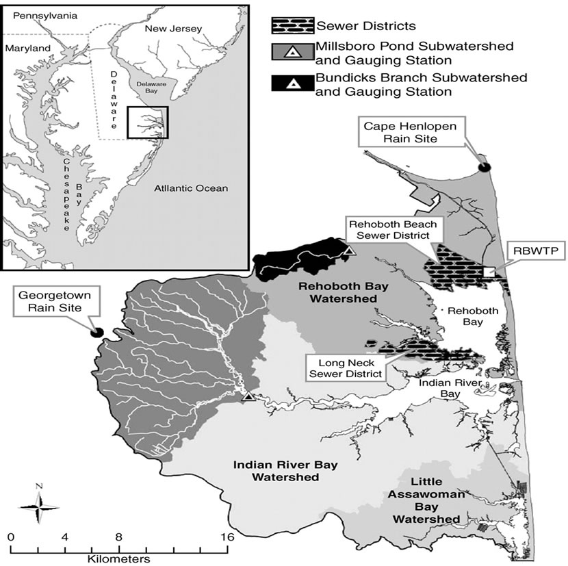
Figure 1. Location of millsboro pond watershed (copied from [9]).
cides deposition in the main channel); and the water or routing phase of the hydrological cycle (which includes water movement, nutrient processes and transport of pesticides from the channel network to the watershed outlet) [11]. Soil water processes include infiltration, runoff, evaporation, plant uptake, lateral flow, and percolation to lower layers, the details of which can be found in SWAT theoretical document [11].
SWAT can also simulate the land management practices and can incorporate very detailed management information. Management practices are broadly divided into agriculture management, water management and urban areas. Some of the management practices in agriculture management include plant growth cycle, timing of fertilizer, type of tillage, pesticide application, and removal of plant bio-mass. The crop model is a simplification of the Erosion Productivity Impact Calculator (EPIC) crop model. Water management includes irrigation, tile drainage, impounded/depressed areas, water transfer, consumptive water use, and loading from point sources. For the urban areas, the model estimates the quantity and quality of the runoff based upon the impervious cover that are either directly connected to the drainage system and not.
2.3. Model Inputs
The terrain elevation data was archived from the United States Geological Survey (USGS) in digital raster form as Digital Elevation Model (DEM). The DEM used in this research was 1-degree DEMs (3- by 3-arc second data spacing), which provides coverage in 1- by 1-degree blocks. The surface water data in the form of reaches data was also downloaded from the National Hydrography Dataset (NHD) developed by USGS based on 1:100,000 scale data. The NHD supersedes USGS Digital Line Graph (DLG) hydrography data and the EPA Reach File Version 3 (RF3).
The soil profile was created from the data downloaded from STATSGO developed by the US National Cooperative Soil Survey. The weather data, which includes precipitation, maximum and minimum temperature, solar radiation, and wind speed, was obtained for the Georgetown station from the Climatology website of the Office of Delaware State. The weather monitoring station is located at latitude of 38°39′ and longitude of 75°27′ at elevation of 50′.
The ground water level data was obtained from the Delaware Geological Society, (http://www.dgs.udel.edu/). The hydrological data was downloaded from the USGS National Water Information System for the station 01484525 at Millsboro Pond outlet At Millsboro. The nutrient data (i.e. nitrogen and phosphorus) for the Millsboro pond outlet was retrieved from the Delaware Inland Bays Water-Quality Database (DIBWQDB) maintained by the Delaware Geological Survey (DGS) [12].
The land use land cover (LULC) was collected from the National Land Cover Database (NLCD) 2001 which is a cooperative effort by the Multi-Resolution Land Characteristics (MRLC) Consortium. The MRLC Consortium is a partnership of federal agencies, consisting of the USGS, the National Oceanic and Atmospheric Administration (NOAA), the U.S. EPA, the U.S. Department of Agriculture (USDA) Forest Service (USFS), the National Park Service (NPS), the U.S. Fish and Wildlife Service (FWS), the Bureau of Land Management (BLM) and the USDA Natural Resources Conservation Service (NRCS).
2.4. Model Evaluation
The model evaluation for hydrology and nutrients was based on two statistical methods – Nash-Sutcliffe coefficient of efficiency (E) [13] and Bias [14]. The NashSutcliffe coefficient of efficiency (NSE) is defined as:
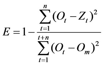 (1)
(1)
where Ot and Zt are observed and simulated values at time t respectively and Om is the mean of observed value. The range of NSE varies from unity to a negative number. Unity means that the model is a perfect fit where as 0 means that the model is no better than the simple average of observed values. A negative value implies that the model is worse than the observed average.
The second goodness-to-fit criterion for the model used was bias. Bias measures the deviation of the simulated value from the observed value, i.e., it measures the tendency of the simulated values to be larger or smaller than the observed value. Mathematically it was calculated as:
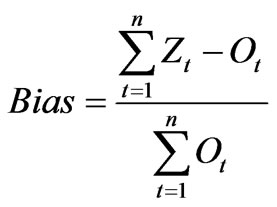 (2)
(2)
2.5. Model Setup
SWAT2000 version used in this study is incorporated in the Version 3.1 of the better assessment science integrating point and nonpoint sources (BASINS). BASINS has its own custom database and GIS interface that allows it to import GIS based physical data from other organizations, making it easier to collect the input data for the SWAT model. It also has many models (one of them being SWAT), which can use the data and the project created to model the watershed.
Maize and soybeans are the major crops grown in this watershed. Two types of tilling methods are used, i.e., chisel-till and no-till. Some farmers practice crop rotation with winter wheat grown in between two crops of soybeans. In addition, some of the agriculture land is irrigated. The agriculture practices that were used are summarized in Table 1. The management practices used for agriculture in the watershed is summarized in Table 2.
Based upon SWAT manual’s recommendations, a threshold of 10% and 15% was used for land use soil respectively. The entire watershed was divided into 37 sub watersheds and 115 HRUs.
Two factors that limited the period for the calibration and validation of the model. Firstly, the land-use/landcover data was from 2001. Thus, it would be more appropriate to work with periods around 2001. Secondly, the observed nutrient information was limited (from 1998 to 2002), thus restricting the period of calibration and validation. The calibration of hydrology was done from January 1997 to December 2000 and the validation was done from January 2001 to December 2002. There was no observed sedimentation data for the Millsboro Pond. The nutrient calibration was done from October 1998 to September 2000 and the validation done for period from October 2000 to October 2001. A two-year “warm up” period from 1995-1997 was allowed.
2.6. Model Calibration
2.6.1. Hydrology
The initial attempts to calibrate the hydrology for the Millsboro watershed were not successful. The stream
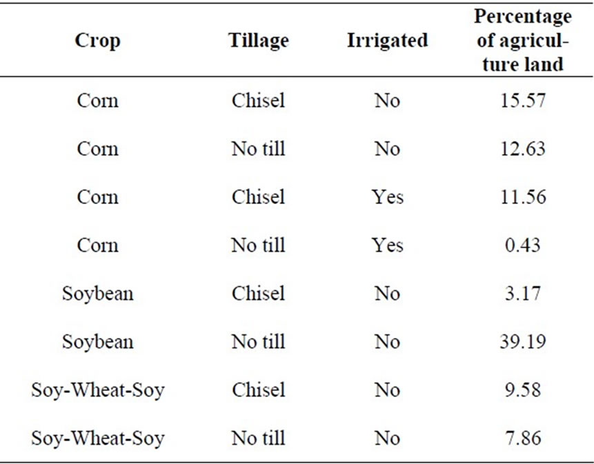
Table 1. Distribution of crop, tillage and irrigation in the watershed.
flow was separated into base flow and surface runoff by using the base flow filter program [15]. The program makes three passes for separating stream flow. In this, the value from the first pass was used. The model constantly under-predicted the stream flow. Although the calibrated base flow trends matched very well with the observed trends, most of the under-predicting was due to the base flow.
Chu and Shirmohammadi [16] demonstrated the role of the subsurface water from outside the watershed. Thus, we decided to carry out a water budget for the watershed to get the contribution of water to the base flow from outside the watershed. As discussed by Chu and Shirmohammadi [16], the water budgeting was carried out on an annual basis. The precipitation was used from the data downloaded from the Climatologist website of the Office of Delaware State for the Georgetown station. The base flow and surface runoff data used was from the output file (output.std) of SWAT. The used evapotranspiration was also estimated by SWAT. The change in soil moisture was considered to be zero for long-term. As discussed in Chu and Shirmohammadi [16], the change in groundwater storage was calculated based on gravity yield of the watershed. The change in groundwater stage was measured by averaging the wellhead measurements from the data collected by the Delaware Geological Survey. An average of eight wells was used to calculate the change in groundwater head for the watershed. The value of gravity yield for the region varies from 0.1 to 0.25, so a value of 0.25 was used. The results of the water balance for the watershed are shown in Table 3. The water balance was done for each year of the calibration. In all but one year, the influence of ground water from outside the watershed on the base flow was prominent. On the average, the ground water from outside the watershed contributed to about 50% of the base flow.
The annual contribution of base flow from out side the watershed was divided into monthly values based on the measured base flow for each month as shown in the following formula:
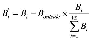 (3)
(3)
where  is the corrected monthly base flow,
  is the monthly measured base flow, and
  is the annual base flow contribution from the outside of the watershed.
Thus, the monthly weighed contribution from outside the watershed was used to correct the base flow.
The results of the hydrology calibration after adjustment of base flow from outside the watershed are shown in Figure 2 and model evaluation results are shown in Table 4. NSE score for base flow increased from 0.44 to 0.59. This helped in better calibration of stream flow for
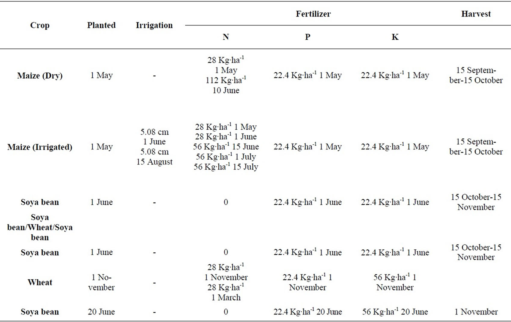
Table 2. Agriculture management practices in the watershed.
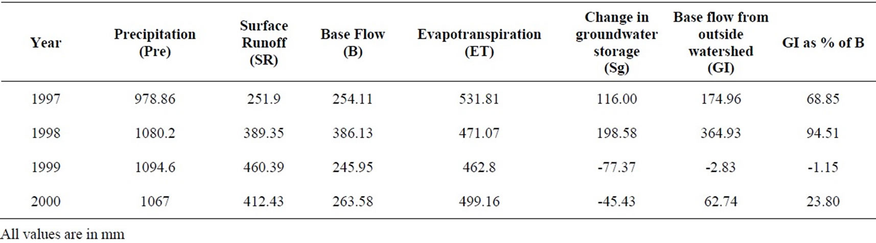
Table 3. Annual water budget for the Millsboro pond watershed.
the watershed. Throughout the period of calibration NSE was low, although if one to two storm events are ignored and the efficiency increases. After removing 2 outliers, the NSE for the surface runoff goes up to 0.55. Thus, except for some storm event runoffs, the model performance was acceptable for simulating the hydrology of the watershed.
From these results, it is evident that although watershed delineation divides land based on surface runoff, it is not necessary that the watershed boundary should coincide with the sub-surface boundaries that govern the flow of groundwater. Thus, for small to medium watersheds, such as the Millsboro Pond watershed, base flow from the adjacent watersheds could have a significant influence. Also, the SWAT model did not simulate the big storm events very well.
2.6.2. Nutrients
For the calibration of nutrients in the Millsboro Pond, we used data from 35 locations for a period of two years. Water samples for nutrient concentrations and flow discharge were measured at the same time and nutrient loads were computed by multiplying the nutrient concentration with the freshwater discharge. The monthly flow rate thus calculated was used as the observed value for the calibration of the nutrients. The observed values for TN were adjusted for the outside flow as discussed by Chu et al. [17]. The results of nutrient calibration are
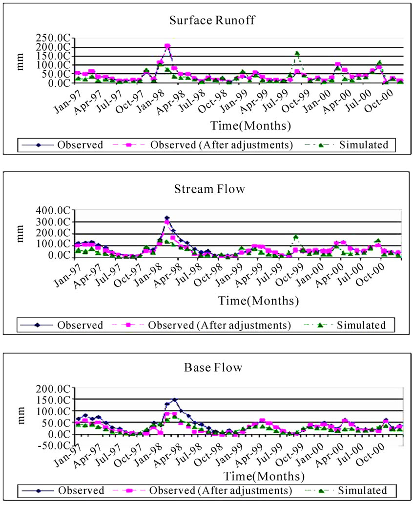
Figure 2. Calibration results for hydrology after adjustment for the base flow from outside the watershed.
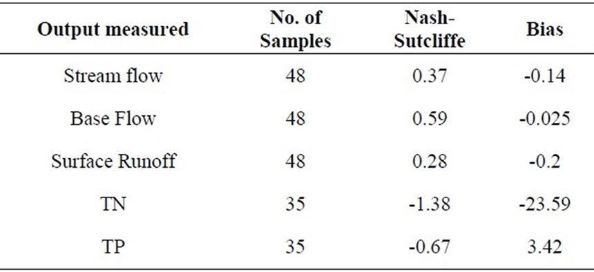
Table 4. Model evaluation results for the calibration for hydrology (January 1997-December 2000) and total nitrogen (TN)/total phosphorus (TP) (October 1998-September 2000) after adjustment for the base flow from outside the watershed.
shown in Figure 3 and the model evaluation results shown in Table 4.
Lack of data for the nutrients adversely influenced the calibration process. Using a single observation value to calculate average nutrient loading for the whole month is bound to generate large amount of error. In addition, the lack of sediment data also impeded a good calibration. The model always under estimated the TN loading and over estimated the TP loading for the watershed. Although there appears to be “lack of data” error, there could be other plausible causes. The model does not account for the role played by atmospheric deposition in TN. Ammonia from the poultry industry and agriculture
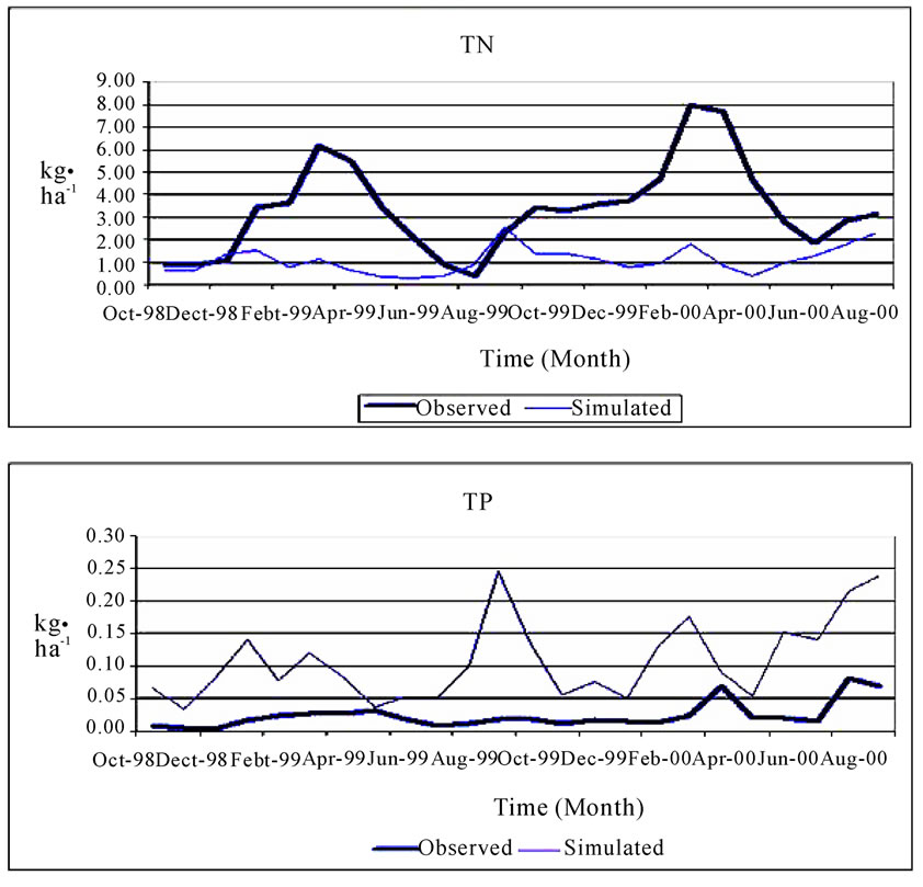
Figure 3. Calibration results for the nutrients after adjustment for the base flow from outside the watershed.
practice contributes significantly to the TN in the region —sometimes up to 33% [2]. This could, to some extent, explain the under estimation of TN loading by the model.
Also, the over-estimation of TP can be explained due to the location of the monitoring station. The sampling station for the nutrients was located in the Millsboro pond. A pond acts as a sedimentation tank for the water flowing into it. Thus measuring nutrients from the pond does not account for the nutrients that settle to the bottom of the pond in the sediment. Since the movement of P in the watershed is mostly due to its adsorption onto the sediments, the measured value of TP will always be underestimated. This can explain the discrepancies between the simulated values and the measured data for the TP loading up to some extent.
The SWAT variables that were modified to achieve the calibration results for hydrology and nutrients are shown in Table 5.
2.7. Model Validation
Validation for the hydrology was done for the period from January 2001 to December 2002 (Table 6). Similar to the calibration of the model for the hydrology, the results were skewed due to the inaccurate simulation of some of the storm events by the model. Overall, the model reasonably predicts the hydrology of the watershed. In terms of the calculated bias, the model gives reasonable prediction for the surface runoff. The validation results for the bias were better than the calibration bias results. The performance of the model to predict nutrient levels (Table 6) was similar to that for calibration for the same reasons as discussed before. Although
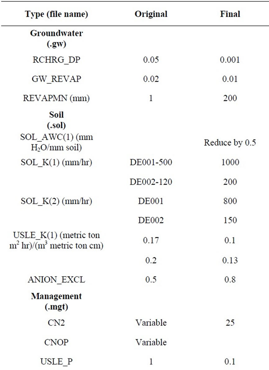
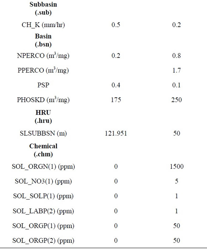
Table 5. SWAT variables modified for the calibration of hydrology and the nutrients for the watershed.
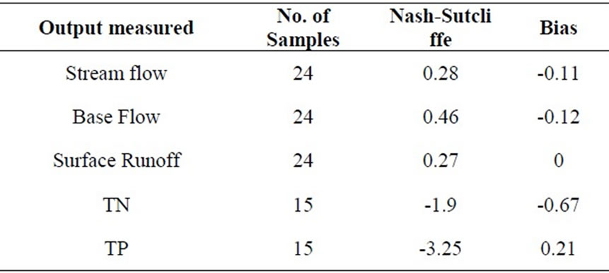
Table 6. Model evaluation results for the validation for hydrology (January, 2001-December, 2002) and total nitrogen (TN)/ total phosphorus (TP) (October, 2000 to September, 2001) after adjustment for the base flow from outside the watershed.
for the validation period, the model simulated TP more accurately. It was a combination of lack of good data and environmental reasons, in addition, the lower bias values suggest that the model accurately simulates the trends in nutrient loading.
2.8. Scenario Setup
Although the nutrient calibration/validation results were not of high quality, the model was still used for scenario studies. This was done because the goal of the study was to measure the percentage change in the nutrient load from the baseline case. The initial results from this study were used as a base line. In general, the model followed the trends in nutrient prediction.
Five scenarios were selected to check their effectiveness to reduce nutrient load in the watershed. Assuming the current land use as a base case scenario, the land use or the agriculture management practices were changed to reflect the following scenarios.
1) Convert all farmland to no-till 2) Convert all farmland to chisel tillage 3) Irrigate agricultural land to increase yield 4) Apply cover crop to the whole agriculture land 5) Convert some land to permanent grassland
3. Results and Discussions
The model was run from October 1998 to October 2001 for nutrients and January 1997 to December 2001 for hydrology. The results from the various scenarios are shown in Figure 4. Table 7 shows the percentage decrease in total TN and TP with the various scenarios, discussed above.
There was 0.5 to 2% reduction in TN and slight increase to 9.5% reductions in TP due to change in tillage practices. The reason for the small change in the TN and TP values is that the existing tillage practice is already 60:40 ratio for no-till versus chisel tillage. The slight decrease in nutrient loading due to irrigation may be
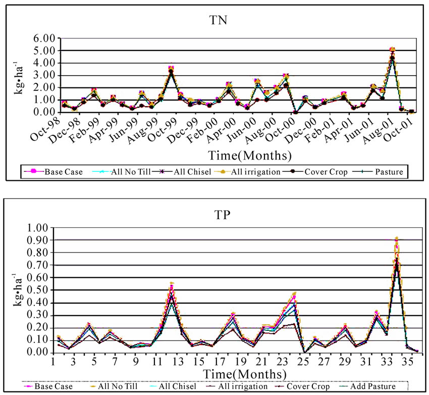
Figure 4. Variation in the nutrients due to simulation of different scenarios.

Table 7. Percentage change in nutrient loading due to simulation of different BMPs and scenarios by SWAT.
attributed to an increase in the yield of the crops, which would imply higher uptake of nutrients (the amount of fertilizer applied is the same) by the plants. This decrease was also not significant. Planting a winter cover crop helped in reducing TN load by roughly 25% and TP load by roughly 27%. The cover crop helped in reducing the erosion and runoff and in increasing uptake of nutrients from the soil. About 38% of the existing agriculture land along the major reaches was converted to grassland (or pastureland) and this helped in reducing TN and TP loading by approximately 12 and 18.5% respectively. Further, pasture also helps in reducing the sheet flow of surface runoff and helps in reducing the erosion. This explains that the larger reduction in TP loading as compared to TN loading.
To reduce the nutrient loading, a combination of measures would have to be implemented. The three most effective measures in decreasing order found in this study were converting agriculture land to forest cover, providing winter cover crops and providing grassland buffer along the reaches. But these measures might not be sufficient to meet the TMDL requirements. None of the above BMPs were able to meet the TMDL requirements. Two extreme scenarios—one replacing agriculture land with deciduous forest, and another replacing agriculture land with high yield forest—hybrid popular were also studied (Table 8). When all of the agriculture land in the watershed converted to forest, it led to significant reduction in nutrient loading, i.e. the TN loading reduced by approximately 46% and the TP loading reduced by approximately 54%. These numbers will go down a little when instead of planning deciduous trees, fast growing poplar trees were planted for harvesting. The TN and TP loading reduced by 42% and 51% respectively.
To achieve the TMDL, as required by the 1972 Clean Water Act there is a need for drastic changes in the land use practice in the watershed. The reductions due to converting agriculture land to forest land are in line with that required by the DNREC to meet the TMDL. Losing agriculture land will influence the region economically, both directly and indirectly. The direct impact of converting agriculture land to forest will result in the loss of income to the farming community. The indirect impact will be loss of local food source for the poultry industry. Agriculture in the watershed is fully integrated with the economic activity of the region – the maize and soybeans grown in the watershed provide the feed for the chicken farms, which is the major industry in southern Delaware. Thus, for an effective solution for reducing nutrient loading in the watershed, along with the BMPs, the economic model of the region also needs to be addressed. To convert existing agriculture land to forest without adversely influencing the income generation of the region, maize and soybeans farming can be replaced by tree farming. The demand for bio fuel for the nation is growing very fast. The technology for production of bio fuel from wood cellulose is improving [18-20] thus making it more efficient (and hence more economically lucrative). Fast growing trees like poplar can be harvested with proper forest management to provide cellulose for the bio fuels. Bio fuel from cellulose is more energy efficient, has
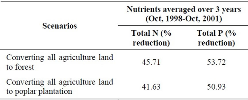
Table 8. Percentage change in nutrient loading due to simulation of two extreme scenarios by SWAT.
less impact on food production, and has less environmental impact than bio fuel from maize or soybeans [18-21].
Young growing trees also uptake large quantities of nutrients from the soil, helps in reducing the nutrient loads in the watershed [22]. Thus, a proper balance among agriculture land, tree farming and buffer grassland can be very effective in reducing the nutrient loading. The tree buffers along the streams (except for immediately next to the water body) can provide a dual purpose of providing its buffering services [23] and also providing raw material for bio fuels. The forest cover also helps in reducing the greenhouse effect by providing larger forest cover to sequester carbon dioxide from the atmosphere. This can provide the region with extra carbon credits that can be traded in a regional/global market in the future. Delaware is one of the participants in the Regional Greenhouse Gas Initiative, which is a cooperative effort of ten states from northeast and Mid-Atlantic to cap and trade carbon emissions [24]. This too can help in the economy of the region [25].
4. Conclusions
This research used SWAT model to evaluate five land use/agriculture practice scenarios in the Millsboro Pond watershed of the Inland Bays Basin in Southern Delaware. The evaluation of the five scenarios showed that they alone were not able to meet the TMDLs requirements as set by the state. Along, with these scenarios, some land use change, like converting agriculture land to tree cover, may be required. This could impact the economy of the region. Hence, to achieve nutrient reduction goals, an economic model that includes land use changes such as managed forests may need to be considered.
5. Acknowledgements
We would like to express our gratitude to Dr. J. T. Sims, Director of the Institute of Soil and Environmental Quality and Maria C. Pautler, Program Coordinator of the Institute of Soil and Environmental Quality for providing us with the opportunity and funding to conduct this research.
REFERENCES
- J. Larsen, “Dead Zones Increasing in World’s Coastal Waters,” Earth Policy Institute, 16 June 2004. http://www. earth-policy.org/Updates/Update41.htm
- Delaware Department of Natural Resources and Environmental Control, “Inland Bays/Atlantic Ocean Basin Assessment Report,” June 2001.
- Delaware Department of Natural Resources and Environmental Control, 2000. http://www.dnrec.state.de.us/DN REC2000/Library/Misc/InlandBays.pdf
- Delaware Department of Natural Resources and Environmental Control, “Inland Bays Pollution Control Strategy,” April 2007. http://www.dnrec.state.de.us/water2000 /Sections/Watershed/ws/ib_pcs.htm
- Delaware Poultry Industry. http://www.dpichicken.org
- Environmental Protection Agency, “Impaired Waters and Total Maximum Daily Loads,” http://www.epa.gov/owow /tmdl/
- P. W. Gassman, M. R. Reyes, C. H. Green and J. G. Arnold, “The Soil and Water Assessment Tool: Historical Development, Applications, and Future Research Directions,” Transactions of the ASABE, Vol. 50, No. 4, 2007, pp. 1211-2150.
- J. G. Arnold and N. Fohrer, “SWAT2000: Current Capabilities and Research Opportunities in Applied Watershed Modeling.” Hydrological Processes, Vol. 19, 2005, pp. 563-572.
- J. A. Volka, K. B. Savidgeb, J. R. Scudlarkb A. S. Andresc and W. J. Ullman, “Nitrogen Loads through Baseflow, Stormflow, and Underflow to Rehoboth Bay, Delaware,” Journal of Environmental Quality, Vol. 35, August 2006, pp. 1742-1755.
- C. Santhi, R. Srinivasan, J. G. Arnold and J. R. Williams, “A Modeling Approach to Evaluate the Impacts of Water Quality Management Plans Implemented in a Watershed in Texas,” Environmental Modelling & Software, Vol. 21, No. 8, pp. 1141-1157.
- S. L. Neitsch, J. G. Arnold, J. R. Kiniry, J. R. Williams and K. W. King, “Soil and Water Assessment Tool Theoretical Documentation, Version 2000,” Soil and Water Research Laboratory and Blackland Research Center, Grassland, 2002.
- Delaware Geological Survey, “Delaware Inland Bays Tributary Total Maximum Daily Load Water-Quality Database,” 2009. http://www.dgs.udel.edu/Hydrology/Sur faceWater.aspx
- J. E. Nash and J. V. Sutcliffe, “River Flow Forcasting through Conceptual Models Part I—A Discussion of Principles,” Journal of Hydrology, Vol. 10, No. 3, April 1970, pp. 282-290.
- P. O. Yapo, H. V. Gupta and S. Sorooshian, “Multi-Objective Global Optimization for Hydrologic Models,” Journal of Hydrology, Vol. 204, No. 1-4, January 1998, pp. 83-97.
- J. G. Arnold and P. M. Allen, “Automated Methods for Estimating Base Flow and Groundwater Recharge from Stream Flow Records,” Journal of the American Water Resources Association, Vol. 35, No. 2, 1999, pp. 411-424.
- T. W. Chu and A. Shirmohammadi, “Evaluation of the SWAT Model’s Hydrology Component in the Piedmont Physiographic Region of Maryland,” Transactions of the ASAE, Vol. 47, No. 5, 2004, pp. 1523-1538.
- T. W. Chu, A. Shirmohammadi, H. Montas and A. Sadeghi, “Evaluation of the SWAT Model’s Sediment and Nutrient Components in the Piedmont Physiographic Region of Maryland,” Transactions of the ASAE, Vol. 47, No. 4, 2004, pp. 1057-1073.
- United States Department of Energy, “Cellulosic Ethanol Research and Development.,” 2008. http://www.eere.energy.gov/afdc/fuels/ethanol_research.html
- A. E. Farrell, R. J. Plevin, B. T. Turner, A. D. Jones, M. O'Hare and D. M. Kammen, “Ethanol Can Contribute to Energy and Environmental Goals,” Science, Vol. 311, No. 5760, 27 January 2006, pp. 506-508.
- L. R. Lynd, “Overview and Evaluation of Fuel Ethanol from Cellulosic Biomass: Technology, Economics, the Environment, and Policy,” Annual Review of Energy and the Environment, Vol. 21, November 1996, pp. 403-465.
- L. R. Lynd, J. H. Cushman, R. J. Nichols and C. E. Wyman, “Fuel Ethanol from Cellulosic Biomass,” Science, New Series, Vol. 251, No. 4999, 15 March 1991, pp 1318-1323.
- R. Lowrance, R. Todd, J. Fail, O. Hendrickson, R. Leonard and L. Asmussen, “Riparian Forests as Nutrient Filters in Agricultural Watersheds,” BioScience, Vol. 34, No. 6, June 1984, pp. 374-377.
- L. Philip, C. Smythb and S. Boutin, “Quantitative Review of Riparian Buffer Width Guidelines from Canada and the United States,” Journal of Environmental Management, Vol. 70, No. 2, February 2004, pp. 165-180.
- “Regional Greenhouse Gas Initiative,” 2007. http://www. rggi.org
- C. A. Zelek and G. E. Shively, “Measuring the Opportunity Cost of Carbon Sequestration in Tropical Agriculture,” Land Economics, Vol. 79, No. 3, August 2003, pp. 342-354.