Journal of Software Engineering and Applications
Vol.7 No.8(2014), Article
ID:47629,16
pages
DOI:10.4236/jsea.2014.78059
D-IMPACT: A Data Preprocessing Algorithm to Improve the Performance of Clustering
Vu Anh Tran1, Osamu Hirose2, Thammakorn Saethang1, Lan Anh T. Nguyen1, Xuan Tho Dang1, Tu Kien T. Le1, Duc Luu Ngo1, Gavrilov Sergey1, Mamoru Kubo2, Yoichi Yamada2, Kenji Satou2
1Graduate School of Natural Science and Technology, Kanazawa University, Kanazawa, Japan
2Institute of Science and Engineering, Kanazawa University, Kanazawa, Japan
Email: tvatva2002@gmail.com, hirose@se.kanazawa-u.ac.jp, thammakorn.kmutt@gmail.com, lananh257@gmail.com, thodx@hnue.edu.vn, kienltt@hnue.edu.vn, ndluu@blu.edu.vn, gavriloff.sv@gmail.com, mkubo@t.kanazawa-u.ac.jp, youichi@t.kanazawa-u.ac.jp, ken@t.kanazawa-u.ac.jp
Copyright © 2014 by authors and Scientific Research Publishing Inc.
This work is licensed under the Creative Commons Attribution International License (CC BY).
http://creativecommons.org/licenses/by/4.0/


Received 15 May 2014; revised 10 June 2014; accepted 3 July 2014
ABSTRACT
In this study, we propose a data preprocessing algorithm called D-IMPACT inspired by the IMPACT clustering algorithm. D-IMPACT iteratively moves data points based on attraction and density to detect and remove noise and outliers, and separate clusters. Our experimental results on two-dimensional datasets and practical datasets show that this algorithm can produce new datasets such that the performance of the clustering algorithm is improved.
Keywords:Attraction, Clustering, Data Preprocessing, Density, Shrinking

1. Introduction
1.1. Clustering Problem and Data Preprocessing
Clustering is the process of dividing a dataset into partitions such that intracluster similarity is maximized. Although it has a long history of development, there remain open problems, such as how to determine the number of clusters, the difficulty in identifying arbitrary shapes of clusters, and the curse of dimensionality [1] . The majority of current algorithms perform well for only certain types of data [2] . Therefore, it is not easy to specify the algorithm and input parameters required to achieve the best result. In addition, it is difficult to evaluate the clustering performance, since most of the clustering validation indexes are specified for certain clustering objectives [3] . Finding an appropriate algorithm and parameters is very difficult and requires a sufficient number of experimental results. The datasets measured from real systems usually contain outliers and noise, and are, therefore, often unreliable [4] [5] . Such datasets can impact the quality of cluster analysis. However, if the data have been preprocessed appropriately—for example, clusters are well-separated, dense and have no noise—the performance of the clustering algorithms may improve.
Data preprocessing is often used to improve the quality of data. In relation to clustering, popular applications of data preprocessing are normalization, removing noisy data points, and feature reduction. Many studies have used Principal Component Analysis (PCA) [6] to reveal representative factors. Although PCA accounts for as much variance of the data as possible, clustering algorithms combined with PCA do not necessarily improve, and, in fact, often degrade, the cluster quality [7] . PCA essentially performs a linear transformation of the data based on the Euclidean distance between samples; thus, it cannot characterize an underlying nonlinear subspace.
Recent studies have focused on new categories of clustering algorithms which prioritize the application of data preprocessing. Shrinking, a data shrinking process, moves data points along the gradient of the density, generating condensed and widely separated clusters [8] . Following data shrinking, clusters are detected by finding the connected components of dense cells. The data shrinking and cluster detection steps are conducted on a sequence of grids with different cell sizes. The clusters detected at these cells are compared using a cluster-wise evaluation measurement, and the best clusters are then selected as the final result. In CLUES [9] , each data point is transformed such that it moves a specific distance toward the center of a cluster. The direction and the associated size of each movement are determined by the median of the data point’s k nearest neighbors. This process is repeated until a pre-defined convergence criterion is satisfied. The optimal number of neighbors is determined through optimization of commonly used index functions to evaluate the clustering result generated by the algorithm. The number of clusters and the final partition are determined automatically without any input parameters, apart from the convergence termination criteria.
These two shrinking algorithms share the following limitations:
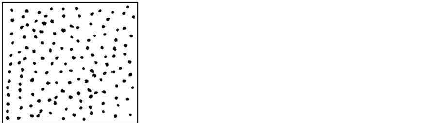
Ÿ The process of shifting toward the median of neighbors can easily fracture the cluster (Figure 1).
Ÿ The direction of the movement vector is not appropriate in specific cases. For example, if the clusters are adjacent and differ highly in density, the median of the neighbors is likely to be located on another cluster.
In addition to the distance, density [10] is a quantity typically considered in clustering. The density represents the distribution of data within a certain distance. Density-based clustering algorithms attempt to find dense regions separated from other regions that satisfy certain criteria. Well-known density-based clustering algorithms include DBSCAN [11] , OPTICS [12] , and DENCLUE [13] . Density clustering algorithms can find arbitrary clusters with high accuracy, but they are highly sensitive to the value of parameters and their accuracy decreases rapidly as the number of attributes increases, especially when dealing with high-dimensional datasets.
1.2. IMPACT Algorithm and the Movement of Data Points
IMPACT [14] is a two phases clustering algorithm which is based on the idea of gradually moving all data points closer to similar data points according to the attraction between them until the dataset becomes self-partitioned. In the first phase of the IMPACT algorithm, the data are normalized and denoised. In the next phase, the IMPACT algorithm iteratively moves data points and identifies clusters until the stop condition is satisfied. The
 (a)
(a) (b)
(b)
Figure 1. Clusters fractured after shrinking. (a) Original dataset; (b) Dataset after shrinking.
attraction can be adjusted by various parameters to handle specific types of data. IMPACT is robust to input parameters and flexibly detects various types of clusters as shown in experimental results. However, there are steps that can be improved in IMPACT, such as noise removal, attraction computation, and cluster identification. Also, IMPACT has difficulties in clustering high dimensional data.
In this study, we propose a data preprocessing algorithm named D-IMPACT (Density-IMPACT) to improve the quality of the cluster analysis. It preprocesses the data based on the IMPACT algorithm and the concept of density. An advantage of our algorithm is its flexibility in relation to various types of data; it is possible to select an affinity function suitable for the characteristics of the dataset. This flexibility improves the quality of cluster analysis even if the dataset is high-dimensional and non-linearly distributed, or includes noisy samples.
2. D-IMPACT Algorithm
In this section, we describe the data preprocessing algorithm D-IMPACT based on the concepts underlying in the IMPACT algorithm. We aim to improve the accuracy and flexibility of the movement of data points in the IMPACT algorithm by applying the concept of density to various affinity functions. These improvements will be described in the subsequent subsections.
2.1. Movement of Data Points
The main difference between D-IMPACT and other algorithms is that the movement of data points can be varied by the density functions, the attraction functions, and an inertia value. This helps D-IMPACT detect different types of clusters and avoid many common clustering problems. In this subsection, we describe the scheme to move data points in D-IMPACT. We assume that the dataset has m samples and each sample is characterized by n features. We also denote the feature vector of the ith sample by xi.
2.1.1. Density
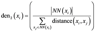
We use two formulae to compute the density of a data point based on its neighbors, which are defined as data points located within a radius Φ. This density is calculated with and without considering the distance from the data point to its neighbors. We define the density δi for the data point xi as
 where
where  is one of following density functions:
 ,
,
 where
where  is the set of neighbors of xi and
  is the number of neighbors. Unlike the density function den1, the density function den2 considers not only the number of neighbors, but also the distance between them to avoid issues relating to the choice of threshold value, Φ. In a practical application, we scale the density to avoid scale differences arising from the use of specific datasets as follows:

2.1.2. Attraction
In our D-IMPACT algorithm, the data points attract each other and one other closer. We define the attraction of data point xi caused by xj as

where  is a function used to compute the affinity between two data points xi and xj. This quantity ignores the affinity between neighbors. The affinity can be computed using the following formulae:


These four formulae have been adopted to improve the quality of the movement process in specific cases. The function aff1, used in IMPACT, considers the distance between two data points only. The function aff2 considers the effect of density on the attraction; highly aggregated data points cause stronger attraction between them than sparsely scattered ones. This technique can improve the accuracy of the movement process. The function aff3 considers the difference between the densities of two data points; two data points attract each other more strongly if their densities are similar. This can be used in the case where clusters are adjacent but have differing densities. The function aff4 is a combination of aff2 and aff3. The parameter p is used to adjust the effect of the distance to the affinity. Attraction is the key value affecting the computation of the movement vectors. For each specific problem in clustering, an appropriate attraction computation can help D-IMPACT to correctly separate clusters.
Under the effect of attraction, two data points will move toward each other. This movement is represented by an n-dimensional vector called the affinity vector. We denote aij as the affinity vector of data point xi caused by data point xj. The kth element of aij is defined as

The affinity vector is a component used to calculate the movement vector.
2.1.3. Inertia Value
To shrink clusters, D-IMPACT moves the data points at the border region of original clusters toward the centroid of the cluster. Highly aggregated data points, usually located around the centroid of the cluster, should not move too far. In contrast, sparsely scattered data points at the border region should move toward the centroid quickly. Hence, we introduce an inertia value to adjust the magnitude of each movement vector. We define the inertia value Ii of data point xi based on its density1 by

2.1.4. Data Point Movement
D-IMPACT moves a data point based on its corresponding movement vector. The movement vector vi of data point xi is the summation of all affinity vectors that affect the data point xi

where aij is the affinity vector. The movement vectors are then adjusted by the inertia value and scaled by s, which is a scaling value used to ensure the magnitude does not exceed a value Φ, as in the IMPACT algorithm. This scaling value is given by

Finally, each data point is moved using

where  is the coordinate of data point xi in the previous iteration, and
  is the coordinate of data point xi in this iteration. We propose the algorithm D-IMPACT based on this scheme of moving data points.
2.2. D-IMPACT Algorithm
D-IMPACT has two phases. The first phase detects noisy and outlier data points, and removes them. The second separates clusters by iteratively moving data points based on attraction and density functions. Figure 2 shows the flow chart of the D-IMPACT algorithm. Since two parameters p and q play similar roles in both IMPACT and D-IMPACT algorithms, they can be chosen according to the instructions in the literature of IMPACT algorithm (in this study, we set p = 2 and q = 0.01). To remove noisy points and outliers, we set the input parameter Thnoise as 0.1, which achieved the best result in our experiments.
2.2.1. Noisy Points and Outlier Detection
First, the distance matrix is calculated. The density of each data point is then calculated by one of the formulae defined in the previous subsection. The threshold used to identify neighbors is computed based on the maximum distance and the input parameter q, and is given by

where ![]() is the largest distance between two data points in the dataset.
is the largest distance between two data points in the dataset.

Figure 2. The outline of the D-IMPACT algorithm.
The next step is noise and outlier detection. An outlier is a data point significantly distant from the clusters. We refer to data points which are close to clusters but do not belong to them to as noisy points, or noise, in this manuscript. Both of these data point types are usually located in sparsely scattered areas, that is, low-density regions. Hence, we can detect them based on density and the distance to clusters. We consider a data point as noisy if its density is less than a threshold Thnoise, and it has at least one neighbor which is noisy or a cluster-point (with the latter defined as a data point whose density is larger than Thnoise). An outlier is a point with a density less than Thnoise that has no neighbor which is noisy or a cluster-point. Figure 3 gives an example of noise and outlier detection.
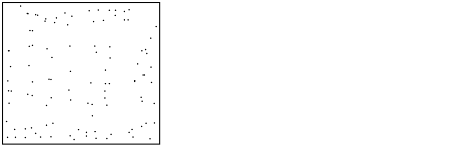
Both outliers and noisy points are output and then removed from the dataset. The effectiveness of this removal is shown in Figure 4. The value ![]() is then recalculated as the dataset has been changed by the removal of noise and outliers. When this phase is completed, the movement phase commences.
is then recalculated as the dataset has been changed by the removal of noise and outliers. When this phase is completed, the movement phase commences.
2.2.2. Moving Data Points
In this phase, the data points are iteratively moved until the termination criterion is met. The distances and the densities are calculated first, after which, we compute the components used to determine the movement vectors: attraction, affinity vector, and the inertia value. We then employ the movement method described in the previous section to move the data points. The movement shrinks the clusters to increase their separation from one another. This process is repeated until the termination condition is satisfied. In D-IMPACT, we adopt various termination criteria as follows:
Ÿ Termination after a fixed number of iterations controlled by a parameter niter.
Ÿ Termination based on the average of the densities of all data points.
Ÿ Termination when the magnitudes of movement vectors have significantly decreased from the previous iteration.
When this phase is completed, the preprocessed dataset is output. The new dataset contains separated and shrunk clusters, with noise and outliers removed.
2.2.3. Complexity
D-IMPACT is a computationally efficient algorithm. The cost of computing m2 affinity vectors is . The
. The
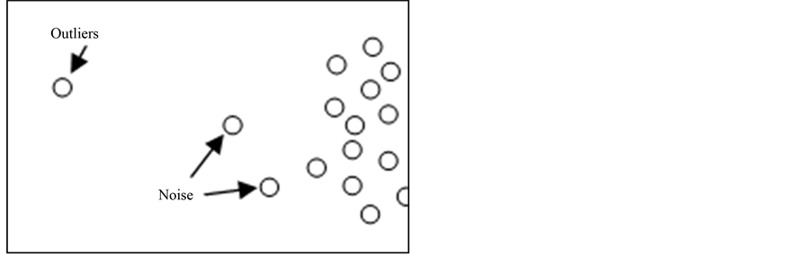
Figure 3. Illustration of noisy points and outliers.
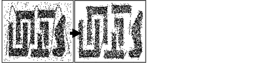
Figure 4. Illustration of the effect of noise removal in D-IMPACT.
complexity of the computation of movement vectors is . Therefore, the overall cost of an iteration is
 . We see, based on our experiments, that the number of iterations is usually small and does not have significant impact on the overall complexity. Therefore, the overall complexity of D-IMPACT is
 .
.
We measured the real processing time of D-IMPACT on 10 synthetic datasets. For each dataset, the data points were randomly located (uniformly distributed). The sizes of the datasets varied from 1000 to 5000 samples. These datasets are included in the supplement to this paper. We compared D-IMPACT with CLUES using these datasets. D-IMPACT was employed with the parameter niter set to 5. For CLUES, the number of neighbors was set to 5% of the number of samples and the parameter itmax was set to 5. The experiments were executed using a workstation with a T6400 Core 2 Duo central processing unit running at 2.00 GHz with 4 GB of random access memory. Figure 5 shows the advantage in speed of D-IMPACT in relation to CLUES.
3. Experiment
In this section, we compare the effectiveness of D-IMPACT and the shrinking function of CLUES (in short, CLUES) on different types of datasets.
3.1. Datasets and Method
3.1.1. Two-Dimensional Datasets
To validate the effectiveness of D-IMPACT, we used different types of datasets: two dimensional (2D) datasets taken from the Machine Learning Repository (UCI) [15] , and a microarray dataset. Figure 6 shows the 2D datasets used.
The 2D datasets are DM130, t4.4k, t8.8k, MultiCL, and Planet. They contain clusters with different shapes, densities and distributions, as well as noisy samples. The DM130 dataset has 130 data points: 100 points are generated randomly (uniformly distributed), and then three clusters, where each cluster comprises ten data points, are added to the top-left, top-right and bottom-middle area of the dataset (marked by red rectangles in Figure 6(a)). The MultiCL dataset has a large number of clusters (143 clusters) scattered equally. Two datasets, t4.8k and t8.8k [16] , used in the analysis of the clustering algorithm Chameleon [17] , are well-known datasets for clustering. Both contain clusters of various shapes and are covered by noisy samples. Clusters are chained by the single-link effect in the t4.8k dataset. The clusters of the Planet dataset are adjacent, but differ in density. These datasets encompass common problems in clustering.
3.1.2. Practical Datasets
The practical datasets are more complex than the 2D datasets, i.e., the high dimensionality can greatly impact the usefulness of the distance function. We used the Wine, Iris, Water-treatment plant (WTP), and Lung cancer (LC) datasets from UCI, as well as the dataset GSE9712 from the Gene Expression Omnibus [18] to test D-IMPACT and CLUES on high-dimensional datasets. The datasets are summarized in Table1 The Iris dataset
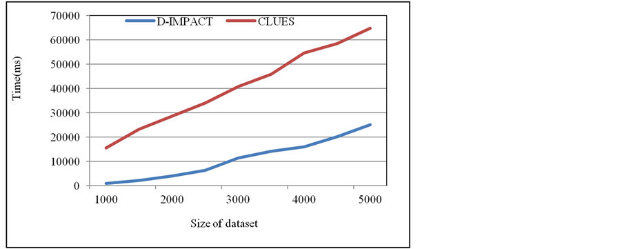
Figure 5. Processing times of D-IMPACT and CLUES on test datasets.
 (a)
(a)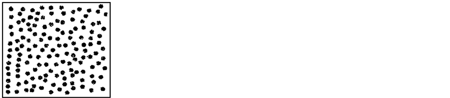 (b)
(b) (c)
(c)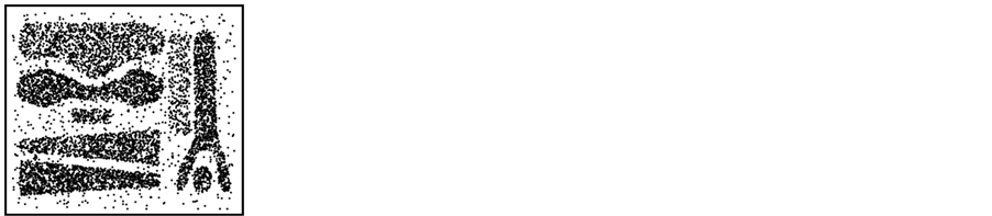 (d)
(d)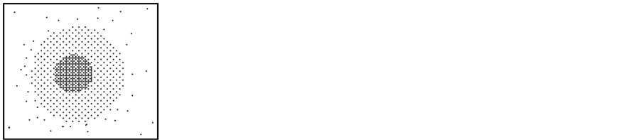 (e)
(e)
Figure 6. Visualization of 2D datasets. a) DM130; b) MultiCL; c) t4.8k; d) t8.8k; e) Planet.

Table 1. Datasets used for experiments.
contains three classes (Iris Setosa, Iris Versicolor, Iris Virginica), each with 50 samples. One class is linearly separable from the other two; the latter are not linearly separable from each other. The Wine dataset (178 samples, 13 attributes), which are the results of chemical analysis of wines grown in the same region in Italy, but derived from three different cultivars, include three overlapping clusters. The WTP dataset (527 samples, 38 attributes) includes the record of the daily measures from sensors in an urban waste water-treatment plant. It is an imbalanced dataset—several clusters have only 1 - 4 members, corresponding to the days that have abnormal situations. The lung cancer (LC) dataset (32 samples, 56 attributes) describes 3 types of pathological lung cancers. Since the Wine, WTP, and LC datasets have attributes within different ranges, we perform scaling to avoid the domination of wide-range attributes. The last dataset we use is a gene expression dataset, GSE9712, which contains expression values of 22,283 genes from 12 radio-resistant and radio-sensitive tumors.
3.1.3. Validating Methods
For a fair comparison, we employed CLUES implemented in R [19] and varied the number of neighbors k (from 5% to 20% of the number of samples) for different datasets. For D-IMPACT, according to the instructions and the experimental results in the literature of IMPACT algorithm, we used the default parameter set (q = 0.01, p = 2, aff1, den1, Thnoise = 0, niter = 2) with some modifications. The complete parameter set is described in Table2 We compared the differences between the preprocessed datasets and the original datasets using 2D plots. However, it is difficult to visualize the high-dimensional datasets using only 2D plots. For this reason, we compared the two algorithms by using a plot showing several combinations of features. Further, to evaluate the quality of the preprocessing, we compared the clustering results for the datasets preprocessed by D-IMPACT and CLUES. We used two evaluation measures, the Rand Index and adjusted Rand Index (aRI) [20] . Hierarchical agglomerative clustering (HAC) was used as the clustering method [10] . We used the Wine, Iris, and GSE9712 datasets to validate the clustering results, and the WTP and LC datasets to validate the ability of D-IMPACT to separate outliers from clusters.
3.2. Experimental Results of 2D Datasets
The results of D-IMPACT and CLUES on 2D datasets DM130, MultiCL, t4.8k, t8.8k, and Planet are displayed and analyzed in this section.
Clusters in the dataset DM130 are difficult to recognize since they are not dense or well separated. Therefore, we set the p to 4 and run D-IMPACT for longer (niter = 3). The D-IMPACT algorithm shrinks the clusters correctly and retains structures of the original dataset (Figure 6(a) and Figure 7(a)). CLUES, with the number of neighbors k varied from 10 to 30, degenerated the clusters into a number of overlapped points and caused a loss of the global structure (Figure 7(b)).
 (a)
(a)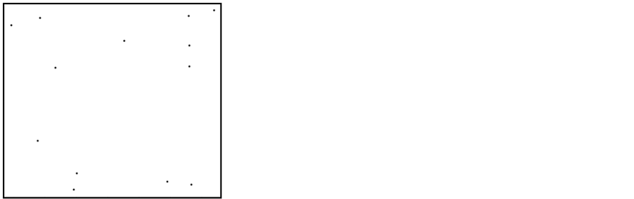 (b)
(b)
Figure 7. Visualization of the dataset DM130 preprocessed by D-IMPACT and CLUES. a) D-IMPACT; b) CLUES.
Table 2. Parameter sets of D-IMPACT for experiments.
The shrinking process may merge clusters incorrectly since clusters in the dataset MultiCL are dense and closely located. Hence, we used the density function den2 and the affinity function aff2, which emphasizes the density, to preserve the clusters. The result is shown in Figure 8. D-IMPACT correctly shrunk the clusters (Figure 8(a)), yet CLUES merged some clusters incorrectly due to issues relating to the choice of k (Figure 8(b)).
In relation to the two datasets t4.8k and t8.8k, D-IMPACT and CLUES are expected to remove noise and shrink clusters. We set q = 0.03 and Thnoise = 0.1 to detect carefully noise and outliers. The results of D-IMPACT are shown in Figure 9; the majority of noise was removed, and clusters were shrunk and separated. We then tested CLUES on the t4.8k dataset. Since the clusters in t4.8k are heavily covered by noise, we tested CLUES on the dataset whose noise was removed by D-IMPACT for a fair comparison. The value k is varied to test the parameter sensitivity of CLUES. Figure 10 shows different results due to this parameter sensitivity.
To separate adjacent clusters in the dataset Planet, we used the function aff3, which considers the density difference. The parameter q is set to 0.05, since the data points are located near each other. We used den2 and p = 4 to emphasize the distance and density. The results are shown in Figure 11. As shown, D-IMPACT clearly outperformed CLUES.
3.3. Experimental Results of Practical Datasets
3.3.1. Iris, Wine, and GSE9712 Datasets
To avoid the domination of wide-range features, we scaled several datasets (Scale = true). In the case of Wine, we had to modify the inertiavalue and use p = 4 to emphasize the importance of nearest neighbors. We used HAC to cluster the original and preprocessed Iris and Wine datasets, and then validated the clustering results with aRI. A higher Rand Index score indicates a better clustering result. The Iris dataset was also preprocessed using a PCA-based denoising technique. However, the distance matrices before and after applying PCA are
 (a)
(a) (b)
(b)
Figure 8. Visualization of the dataset MultiCL preprocessed by D-IMPACT and CLUES. a) D-IMPACT; b) CLUES.
 (a)
(a)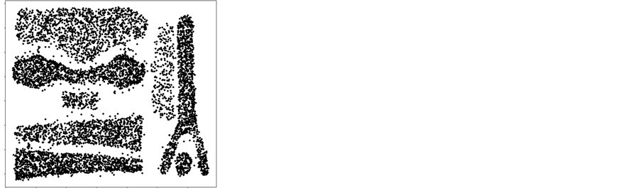 (b)
(b)
Figure 9. Visualization of two datasets t4.8k and t8.8k preprocessed by D-IMPACT. a) t4.8k; b) t8.8k.
 (a)
(a) (b)
(b)
Figure 10. Visualization of the dataset t4.8k preprocessed by CLUES using different values of k based on the size of the dataset. a) k = 80 (1%); b) k = 160 (2%).
 (a)
(a) (b)
(b)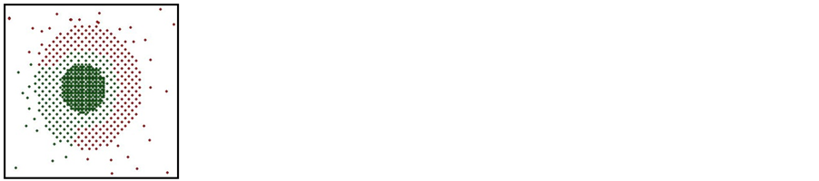 (c)
(c)
Figure 11. Visualization of the dataset Planet preprocessed by D-IMPACT and CLUES. a) Preprocessed by D-IMPACT. Two clusters are separated; b) Preprocessed by CLUES; c) Clustering result using HAC on the dataset in b), indicating that CLUES shrinks clusters incorrectly.
nearly the same (using 2, 3, or 4 principal components (PCs)). Therefore, the clustering results of HAC for the dataset preprocessed by PCA are at most the same result as that of the original dataset, which depends on the number of PCs used (aRI score ranged from 0.566 to 0.759). Table 3 shows the aRI scores of clustering results of HAC on original datasets and datasets preprocessed by D-IMPACT and CLUES. The effectiveness was dependent on the datasets. In the case of Iris, D-IMPACT greatly improved the dataset, particularly as compared with CLUES. However, for the Wine dataset, CLUES achieved the better result. This is due to the overlapped clusters in the Wine dataset are undistinguishable using affinity function. In addition, we calculated aRI scores to compare clustering results obtained by the clustering algorithms IMPACT and D-IMPACT. For the Iris dataset, the best aRI score achieved by IMPACT was 0.716, which was greatly lower than the best aRI score by D-IMPACT (0.835). For the Wine dataset, the best aRI score by IMPACT was 0.897, which was slightly lower than the best aRI score by D-IMPACT (0.899). These results show that the movement of the data points was improved in D-IMPACT compared to the IMPACT algorithm. The GSE9712 dataset is high-dimensional and has a small number of samples. Due to the curse of dimensionality and the noise included in microarray data, it is very difficult to distinguish clusters based on the distance matrix. We performed D-IMPACT and CLUES on this dataset to improve the distance matrix, and then applied the clustering algorithm HAC. D-IMPACT clearly outperformed CLUES since CLUES greatly decreased the quality of the cluster analysis.
We also performed k-means clustering [10] on these datasets. We performed 100 different initializations for each dataset. The clustering results also favored D-IMPACT. Table 4 shows the best and average scores (in brackets) of the experiments. In addition, using Welch’s two sample t-test, the stability of the clustering result on D-IMPACT increased; the p-values between two experiments (100 runs of k-means for each experiment) of the original dataset, CLUES, and D-IMPACT were 0.490, 0.365 and 0.746, respectively. Since the p-value of the t-test is the confidence of the alternative “the two vectors have different means”, a higher p-value indicates more stable clustering results.
Table 3. The Index scores of clustering results using HAC2 on the original and preprocessed datasets of Iris and Wine. The best scores are in bold.
Table 4. Index scores of clustering results using k-means on original and preprocessed datasets of IRIS and Wine. The best scores are in bold.
To clearly show the effectiveness of the two algorithms, we visualized the Iris and Wine datasets preprocessed by D-IMPACT and CLUES as shown in Figure 12. Since Wine has 13 features (i.e. 78 subplots are required to visualize all the combinations of the 13 features), we only visualize the combinations for the first four features, using 2D plots (Figure 13). D-IMPACT successfully separated two adjacent clusters (blue and red) in the Iris dataset. D-IMPACT also distinguished overlapping clusters in the Wine dataset. We marked the separation created by D-IMPACT with red-dashed ovals in Figure 13. This shows that D-IMPACT worked well with overlapped clusters. CLUES degenerated the dataset into a number of overlapped points. This caused the loss of cluster structures and reduced the stability of clusters in the dataset (Figure 14). Therefore, the use of k-means created different clustering results during the experiment.
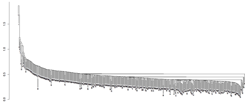
3.3.2. Water-Treatment Plant and Lung Cancer Datasets
To validate the outlier separability, we tested CLUES and D-IMPACT on the WTP and LC datasets. The WTP dataset has small clusters (1 - 4 samples for each cluster). Using aff2, we can reduce the effect of the affinity to these minor clusters. We show the dendrogram of HAC clustering results (using single-linkage) on the original and preprocessed dataset of WTP in Figure 15. In the dataset preprocessed by D-IMPACT, several minor clusters are more distinct than the major clusters (Figure 15(b)). In addition, the quality of the dataset was improved after preprocessing by D-IMPACT; the clustering result using k-means (100 runs) on the dataset preprocessed by D-IMPACT achieved average aRI = 0.217, while the clustering result on the original dataset had average aRI = 0.120. CLUES merged minor clusters during shrinking and, therefore, the clustering result was bad (average aRI = 0.114). To compare the outlier detection capability of D-IMPACT and CLUES, we calculated the Rand Index scores for only minor clusters. The resulting dataset preprocessed by D-IMPACT achieved Rand Index = 0.912, while CLUES had Rand Index = 0.824. In addition, in the clustering result on the dataset preprocessed by D-IMPACT, 8 out of 9 minor clusters were correctly detected. In contrast, no minor cluster was correctly detected when using CLUES.
The lung cancer (LC) dataset was used by R. Visakh and B. Lakshmipathi to validate the outlier detection ability of an algorithm focusing on a constraint based cluster ensemble using spectral clustering, called CCE [21] . The dataset has no obvious noise or outliers. We detected some noise and outlier points by considering the distance to the nearest neighbor and the average distance to the k-nearest neighbors (k = 6) of 32 samples in the LC dataset. We generated a list of candidates for noise and outliers: sample numbers 18, 19, 23, 26, and 29. We then performed HAC with different linkages on the original and preprocessed LC datasets to detect noise and
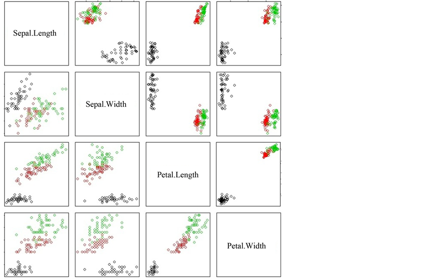
Figure 12. Visualization of the Iris dataset before and after preprocessing by D-IMPACT. Visualization of the original dataset is shown in the bottom-left triangle. Visualization of the dataset optimized by D-IMPACT is shown in the top-right triangle.
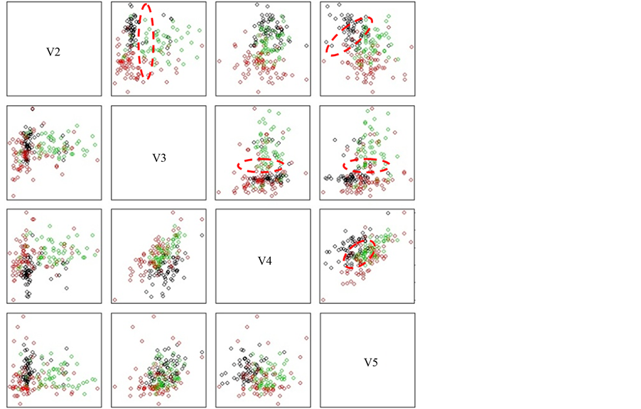
Figure 13. Visualization of the first four features of the Wine dataset before and after preprocessing by D-IMPACT. Visualization of the original dataset is shown in the bottom-left triangle. Visualization of the dataset preprocessed by D-IMPACT is shown in the top-right triangle.
outliers based on the dendrogram. These results were then compared with the reported result of CCE. This was done by calculating the accuracy and precision values. The results in Table 5 clearly show that D-IMPACT outperformed CCE. It also shows the effectiveness of D-IMPACT in relation to outlier detection.
4. Conclusion and Discussion
In this study, we proposed a data preprocessing algorithm named D-IMPACT inspired by the IMPACT clustering algorithm. D-IMPACT moves data points based on attraction and density to create a new dataset where noisy points and outliers are removed, and clusters are separated. The experimental results with different types of datasets clearly demonstrated the effectiveness of D-IMPACT. The clustering algorithm employed on the datasets preprocessed by D-IMPACT detected clusters and outliers more accurately.
Although D-IMPACT is effective in the detection of noise and outliers, there are some difficulties remaining. In the case of sparse datasets (e.g., microarray data and text data), the approach to noise detection based on the density often fails since most of the data, including noise and outlier points, will have a density which equals 1 under our definition. In addition, the distances between data points are not so different due to the curse of dimensionality. In order to overcome this problem, we consider an attraction measure between two data points. The attraction of a noise or outlier point is usually small since it is far from other data points. These problems may be overcome by using the density and attraction information to detect these data point types.
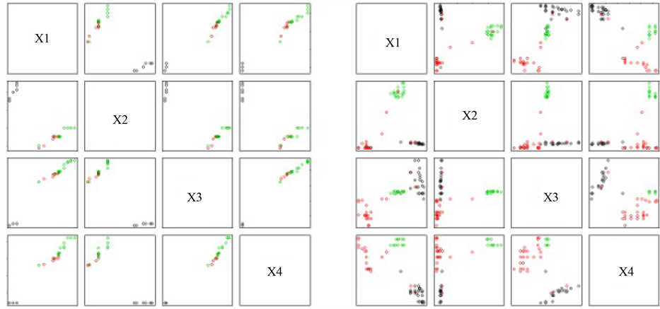 (a) (b)
Figure 14. Visualization of the Iris and Wine datasets preprocessed by CLUES. a) Iris; b) Wine.
Table 5. Accuracy and precision values of noise and outlier detection on the lung cancer dataset.
 (a)
(a)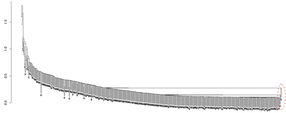 (b)
(b)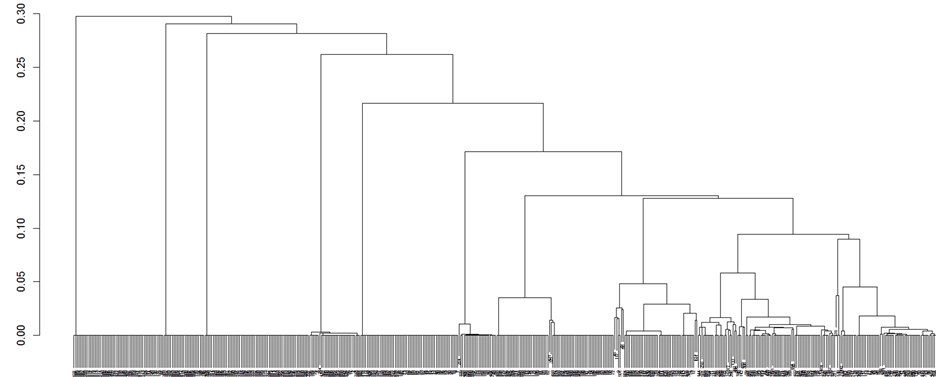 (c)
(c)
Figure 15. Dendrograms of the clustering results on the WTP dataset. a) Dendrogram of the original water-treatment dataset; b) Dendrogram of the water-treatment dataset after being preprocessed by D-IMPACT; c) Dendrogram of the water-treatment dataset after being preprocessed by CLUES.
Availability
The algorithm D-IMPACT is implemented in C++. For readers who are interested in this work, the implementation and datasets are downloadable at [22] .
Acknowledgements
In this research, the super-computing resource was provided by Human Genome Center, the Institute of Medical Science, The University of Tokyo. Additional computation time was provided by the super computer system in Research Organization of Information and Systems (ROIS), National Institute of Genetics (NIG).
References
- Berkhin, P. (2002) Survey of Clustering Data Mining Techniques. Technical Report, Accrue Software, San Jose.
- Murty, M.N., Jain, A.K. and Flynn, P.J. (1999) Data Clustering: A Review. ACM Computing Surveys, 31, 264-323. http://dx.doi.org/10.1145/331499.331504
- Halkidi, M., Batistakis, Y. and Vazirgiannis, M. (2001) On Clustering Validation Techniques. Journal of Intelligent Information Systems, 17, 107-145. http://dx.doi.org/10.1023/A:1012801612483
- Golub, T.R., et al. (1999) Molecular Classification of Cancer: Class Discovery and Class Prediction by Gene Expression Monitoring. Science, 286, 531-537. http://dx.doi.org/10.1126/science.286.5439.531
- Quinn, A. and Tesar, L. (2000) A Survey of Techniques for Preprocessing in High Dimensional Data Clustering. Proceedings of the Cybernetic and Informatics Eurodays.
- Abdi, H. and Williams, L.J. (2010) Principal Component Analysis. Wiley Interdisciplinary Reviews: Computational Statistics, 2, 433-459. http://dx.doi.org/10.1002/wics.101
- Yeung, K.Y. and Ruzzo, W.L. (2001) Principal Component Analysis for Clustering Gene Expression Data. Bioinformatics, 17, 763-774. http://dx.doi.org/10.1093/bioinformatics/17.9.763
- Shi, Y., Song, Y. and Zhang, A. (2005) A Shrinking-Based Clustering Approach for Multidimensional Data. IEEE Transaction on Knowledge Data Engineering, 17, 1389-1403. http://dx.doi.org/10.1109/TKDE.2005.157
- Chang, F., Qiu, W. and Zamar, R.H. (2007) CLUES: A Non-Parametric Clustering Method Based on Local Shrinking. Computational Statistics & Data Analysis, 52, 286-298. http://dx.doi.org/10.1016/j.csda.2006.12.016
- Jain, A.K. and Dubes, R.C. (1988) Algorithms for Clustering Data. Prentice Hall, Upper Saddle River.
- Ester, M., Kriegel, H.P., Sander, J. and Xu, X. (1996) A Density-Based Algorithm for Discovering Clusters in Large Spatial Databases with Noise. Proceedings of the 2nd International Conference on Knowledge Discovery and Data mining, 226-231.
- Ankerst, M., Breunig, M.M., Kriegel, H.P. and Sander, J. (1999) OPTICS: Ordering Points to Identify Clustering Structure. Proceedings of the ACM SIGMOD Conference, 49-60.
- Hinneburg, A. and Keim, D. (1998) An Efficient Approach to Clustering in Large Multimedia Databases with Noise. Proceeding 4th International Conference on Knowledge Discovery & Data Mining, 58-65.
- Tran, V.A., et al. (2012) IMPACT: A Novel Clustering Algorithm Based on Attraction. Journal of Computers, 7, 653-665. http://dx.doi.org/10.4304/jcp.7.3.653-665
- The UCI Machine Learning Repository. http://archive.ics.uci.edu/ml/datasets
- Karypis Lab Datasets. http://glaros.dtc.umn.edu/gkhome/fetch/sw/cluto/chameleon-data.tar.gz
- Karypis, G., Han, E.H. and Kumar, V. (1999) CHAMELEON: A Hierarchical Clustering Algorithm Using Dynamic Modeling. Computer, 32, 68-75. http://dx.doi.org/10.1109/2.781637
- Radioresistant and Radiosensitive Tumors and Cell Lines. http://www.ncbi.nlm.nih.gov/geo/query/acc.cgi?acc=GSE9712
- Chang, F., Qiu, W., Zamar, R.H., Lazarus, R. and Wang, X. (2010) Clues: An R Package for Nonparametric Clustering Based on Local Shrinking. Journal of Statistical Software, 33, 1-16.
- Hubert, L. and Arabie, P. (1985) Comparing Partitions. Journal of Classification, 2, 193-218.
- Visakh, R. and Lakshmipathi, B. (2012) Constraint Based Cluster Ensemble to Detect Outliers in Medical Datasets. International Journal of Computer Applications, 45, 9-15.
- D-IMPACT Preprocessing Algorithm. https://sourceforge.net/projects/dimpactpreproce/
NOTES

1In the case of very sparse datasets, neighbor detection based on a scanning radius usually fails. Therefore, all data points will have a density equal to 1. Hence, we replace the formula used to compute the inertia value with 

2We used the linkage that achieved the best result on the original dataset to perform clustering on the preprocessed dataset. These were average linkage for Iris, complete linkage for Wine dataset, and single linkage for GSE9712.